Statistical Assessment of Biogenic Risk for the Human Population from New Viral Infections Based on COVID-19

Introduction. Understanding the epidemic curve and spatiotemporal dynamics of SARS-CoV-2 virus spread is necessary, firstly, to assess its epidemiological characteristics. In addition, it allows us to work out and implement measures to counter the spread of coronavirus infection (COVID-19), rationally allocate resources. The work objective is to create a mathematical model of the epidemic process, which makes it possible to explain the observed dynamics, predict the spread of infection and assess the reliability of such forecasts. COVID-19 is a new disease, so it is being studied through detailed monitoring of infections and mortality. The results are interpreted using mathematical models and related analytical approaches [1–2]. Knowledge of the evolutionary patterns and numerical indicators of epidemic diseases makes it possible to stop the process in a timely manner, using official medical and other organizational resources [3–4]. Reliable factual information on the incidence of COVID-19 and related mortality on a global scale [5] is published on worldometers.info[1] (the period from 12.02.2020 to 22.09.2021 is considered). The use of these data reduces the errors of regional and time monitoring to some extent, but may prevent the identification of local dynamic parameters of the process. However, the duration of the observations recorded in [5] allows us to hope that this disadvantage is offset by the time series analysis technique [6].

The available data on the dynamics of morbidity and mortality of Covid-positive patients from 12.02.2020 to 22.09.2021 are taken from worldometers.info. Based on them, the authors have constructed the diagrams (Fig. 1–2).

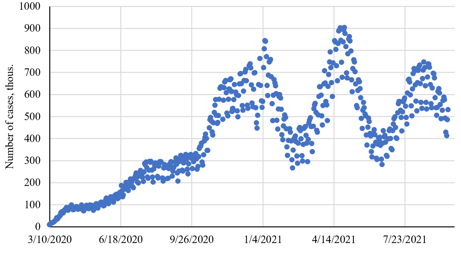
Fig. 1. Data on the incidence of COVID-19

The authors set the task to analyze the relationship of mortality (recorded subsequently) with the stage of the pandemic and the level of morbidity. To do this, the initial data were grouped by quarters (3 months). In Figure 2, they are indicated by dots of a certain color. This approach visualizes the representation of transformed mortality data, in which the moments of death do not explicitly appear.

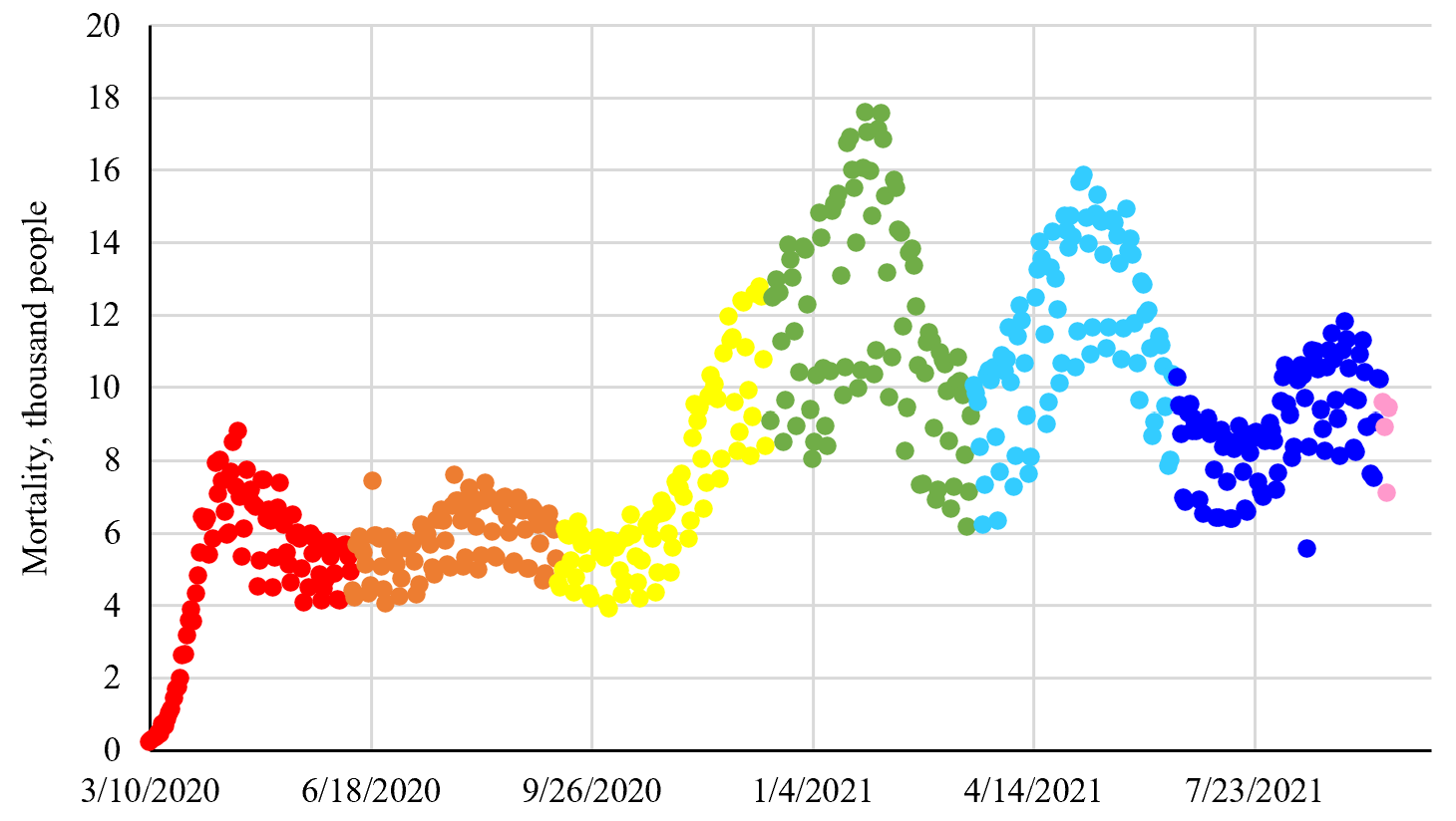
Fig. 2. Actual data on mortality of Covid-positive patients. The red dots indicate the pandemic period from 12.02.20 to 9.06.20; orange — from 10.06.20 to 10.09.20; yellow — from 11.09.20 to 14.12.20; green — from 16.12.20 to 17.03.21; light blue — from 18.03.21 to 17.06.21; blue — from 18.06.21 to 18.09.21; lilac — from 19.09.21 to 22.09.21

Materials and Methods. The data considered are a composition of regular and random components. In the regular ones, aperiodic and periodic components are distinguished. Accordingly, the analysis, interpretation and forecasting in this case are performed by classical means of time series research [6]. We are talking about the sequential allocation of the trend (aperiodic component), cyclic and noise (random) components. Each of them is mathematically characterized by amplitude and (or) time parameters [7]. We will sequentially isolate these components from the actual data, and then describe the results.

The classical technique of studying time series Ф(t) was chosen as a mathematical tool for analyzing and predicting the dynamics of COVID-19 [6]. It is implemented in several stages, which are aimed at consistently identifying regular P(t), oscillatory П(t) and random   components of the trend. In this case, as a rule, the hypothesis is taken into account that the time average value of the last two components of the time series is zero

                                                                         Ф(t) = P(t) + П(t) + , (1)

that is , the ratio is fulfilled:

 (2) 

The regular component P(t) is extracted first. The algorithmic basis here is the theory of function approximation [7]. It is based on the idea of finding a curve of a given type, as close as possible to a cloud of points displaying a time series. In this case, it is required to successfully choose a template for approximating a series function. On the one hand, this is an exceptionally creative task. On the other hand, it requires deep knowledge in the field of mathematical analysis. Then the regular component is excluded from (1) and the combination  is analyzed.

Important characteristics of such a residual term are period and form [8]. The technique of correlation and Fourier analysis is used to identify the period of the leaving П(t). In the framework of autocorrelation analysis, the period of the function П(t) is the value τ satisfying the condition

(3)

where [0…T] — П(t) value observation interval.

The use of a discrete Fourier transform for the same purpose makes it possible to localize the value of τ in a narrow interval. Knowing τ, it is possible to identify the form of the periodic component, but often researchers limit themselves to the first harmonic.

The final stage is the identification of statistical properties  . For this, the method of moments is the most convenient one [9]. It works like this: the actual noise moments of the series ξ(t) are compared with the moments of the model noise given by the known distribution functions F(ξ). The described scheme for analyzing the time series Ф(t) is shown in Fig. 3.

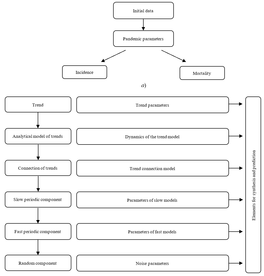
Fig. 3. Analysis of the time series of morbidity and mortality of Covid-positive patients: a — stages according to the focus of research; b — the study algorithm

Results. It is known that any epidemic process in the initial stage is characterized by exponential dynamics in time [10], i.e.

 , (4)

where  — number of cases;  and  — some positive numbers.

Further development of the epidemic may occur according to an optimistic or pessimistic scenario. In the first case, the epidemic reaches a certain peak and comes to naught. The dependence of the number of cases at some point has the form:

, (5)

where A, B, C — coefficients of the model;  — hyperbolic cosine.

This scenario corresponds to the differential equation:

(6)

Here the plus sign is implemented at up to the t* moment, at which . Starting from this moment, the minus sign is implemented in formula (6). According to (6), upon reaching a certain critical number of cases  , the incidence will begin to decrease monotonously.

The pessimistic scenario implies that the epidemic, which initially develops exponentially, also reaches a plateau exponentially over time, i.e. the pathogen remains in the affected population. This can be described by evolutionary dependence

(7)

which corresponds to the differential equation:

(8)

Here  — hyperbolic tangent. In (7) and (8), the multiplier 2 is added for reasons of coincidence of the starting asymptotics, i.e. to fulfill the natural relation:

(9)

The intermediate epidemic scenario combines the elements of the two considered ones and assumes the following stages:

1) primary exponential growth;

2) saturation and subsequent decline;

3) exit to a non-zero plateau.

The dynamics of morbidity in this case is described by the linear conjugation of formulas (5) and (7) with weight D:

(10)

where D — the coefficient reflecting the contribution of an optimistic and pessimistic scenario to the overall process..

Solution (10) corresponds to nonlinear high-order differential equation [11], which we omit because of its bulkiness.

To find the coefficients А, В, С, D, it is necessary to solve mathematical programming problem [12] in its general form:

(11)

where  and t_i are, respectively, the incidence and the moment of its fixation.

Extremum condition (11) corresponds to the generalized epidemic scenario. In particular cases of models (5) and (7), constraints D = 1 or D = 0 should be added to (11).

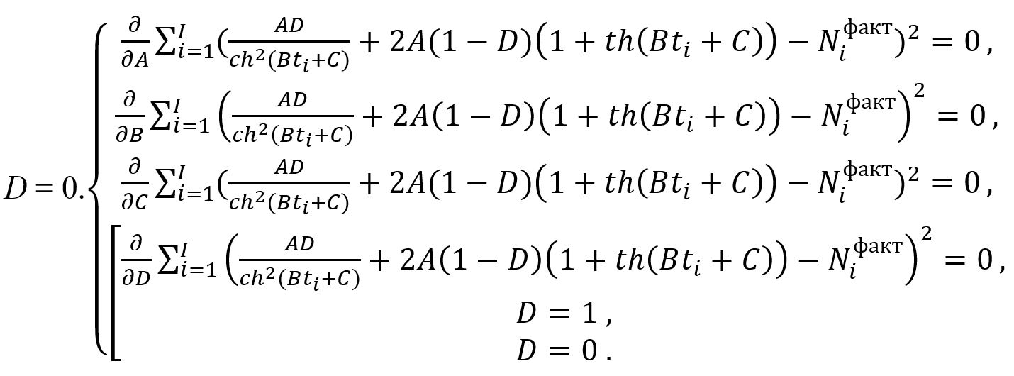(12)

Here  denotes the partial differential. It can also be strictly proved that system (12) is equivalent to an overdetermined system of algebraic equations:

(13)

the variants of which correspond to the described scenarios.

The results of identifying the trend dependence P(t) using the built-in MS Excel functions [13] for all scenarios of epidemic dynamics are shown in Figure 2 and in Table 1.

Table 1

Numerical characteristics of the trend model of COVID-19 morbidity

As it can be seen from the data in the table, generalized model (10) describes the real situation better. However, it has a significant drawback. This is the comparative complexity and inability to explicitly write out nonlinear differential equations that correspond to the dynamics of COVID-19. In this respect, the pessimistic model attracts with its simplicity and, accordingly, the possibilities of improvement.

To identify the oscillatory component in the mortality data for COVID-19 (Fig. 3), we choose the following model. Let us assume that the real data fluctuates near the trend line. In our case, these are models (5)–(6), (7)–(8) and (10) with an amplitude α, a circular frequency β and an initial phase γ. Such a regular model of epidemic dynamics is decomposed and described by equation:

(14)

To find the parameters of oscillatory model (14), it is necessary to solve the following optimization problem [12]              :

(15)

If we consider (15) as a function of the variables α, β, γ, the necessary condition of the extremum takes the form [8]:

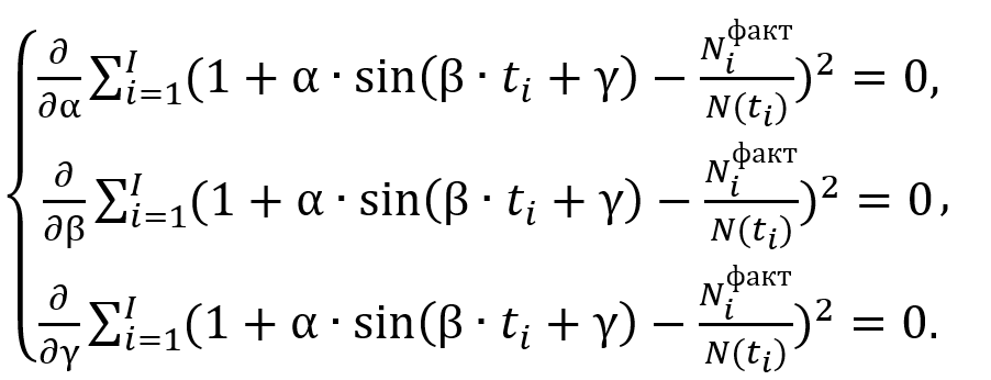(16)

The solution of problem (16) coincides with the solution of the overdetermined system of equations:

(17)

However, the practical implementation of algorithms (16) and (17) is hampered by their instability due to the peculiarities of problem [7]. In this case, the algorithm based on finding the model parameters that provide the best correlation between actual data [9] and the model function   is more stable:

(18)

Solution (18) obtained by means of Excel [9] for variants of model  (5)–(6), (7)–(8) and (10) are given in Table 2.

Table 2

Numerical characteristics of the COVID-19 incidence fluctuation model

Numerical indicators of the adequacy of models ξ and σ presented in Table 2 indicate that the generalized model better corresponds to the actual data. At the same time, it is much more difficult than the pessimistic one with an insignificant improvement in accuracy. Thus, the advantage of the pessimistic model should be recognized. It has the optimal complexity of the mathematical description of the COVID-19 epidemic, allowing for simple interpretation and ease of improvement.

It is important to note that any trend is characterized by a periodicity of 127 ± 0.5 days. This result is in good agreement with the data of autocorrelation and spectral analysis of the oscillation component of    function (Fig. 4). Thus, it is recorded that outbreaks of the disease occur after 124 and 110 days. This means that the disease is seasonal with a period of 1/3 of the year.

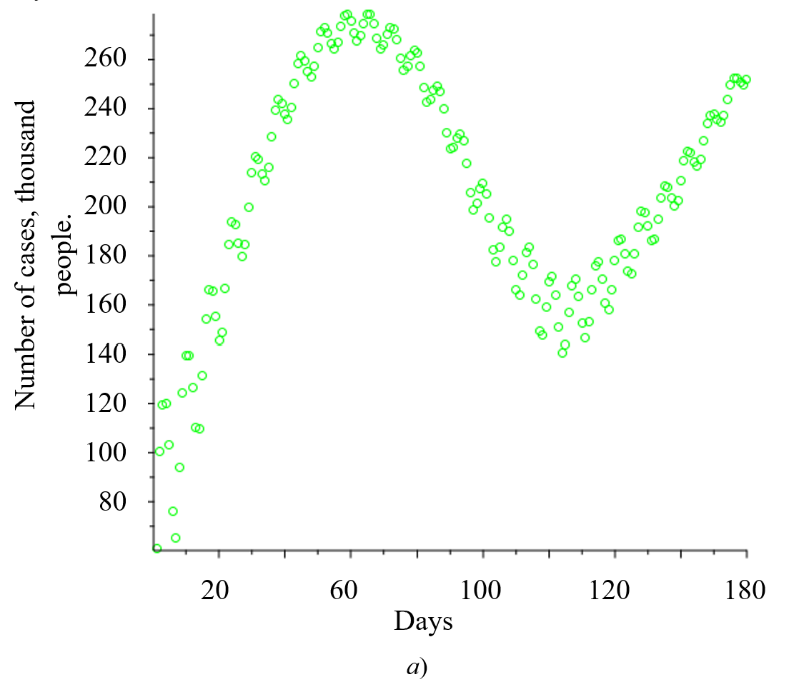
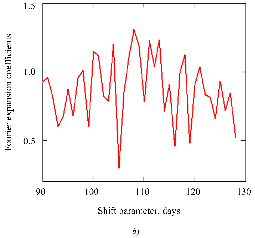
Fig. 4. Data of autocorrelation and spectral analysis of the oscillation component: a — difference in the dynamics of morbidity with a shift by a different number of days; b — coefficients of spectral decomposition of morbidity

Data comparison in Tables 1 and 2 allows us to assess the relative role of the oscillation and noise components. If we consider them independent (orthogonal) and use the well-known ratio , we can make sure that the contributions of the periodic and random components are comparable.

Subtracting the model values of morbidity   from the observed ones  (or vice versa), we allocate the remaining noise component of the model. Figure 5 provides the result for the pessimistic scenario.

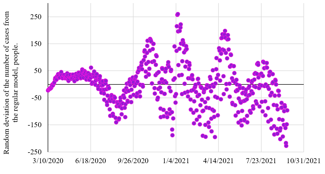
Fig. 5. Noise component in the pessimistic model

Numerical characteristics of data shown in the figure correspond to a normal Gaussian distribution [9] with a mathematical expectation of "zero" and a standard deviation of 80 thousand cases per day, which is confirmed by numerical identification data:

– mathematical expectation M = –2.87;

– standard deviation σ = 79.9;

– Skewness asymmetry = 0.0085;

– Kurtosis excess = 3.51.

Thus, the identification of the mathematical model   performed in this work, presumably, allows predicting morbidity for the entire duration of the epidemic [5].

Similarly, the dynamics of mortality among Covid-positive patients was analyzed from 12.02.2020 to 22.09.2021 (Fig. 3). Given that the lethal outcome is a likely result of infection, it is logical to present a mortality model:

(19)

Or taking into account the approximation of morbidity:

(20)

Here M denotes mortality;  k_leth— the probability of dying from this disease; — the most likely time from infection of a person to his death. We find numeric parameters k_leth and , that appear in mortality patterns (19), by minimizing the functional deviations:

(21)

taking into account natural constraints .

The peculiarity of the solution to problem (21) is that one of the desired variables appears in the upper index of summation. Therefore, we will get the solution to the optimization problem in two stages. The first one is based on a necessary condition for the extremum  :

(22)

for the entire range of . Then we choose a pair of values , that provides the minimum value (21).

It is important to mention that   is assumed to be equal to 150 days. The assumption is due to the fact that the first months of morbidity and mortality statistics [5] do not seem to be sufficiently complete and reliable.

Having solved problem (21), we get:  and  days. The correlation of mortality with morbidity is demonstrated in more detail by the correlogram of the data  (Fig. 6).

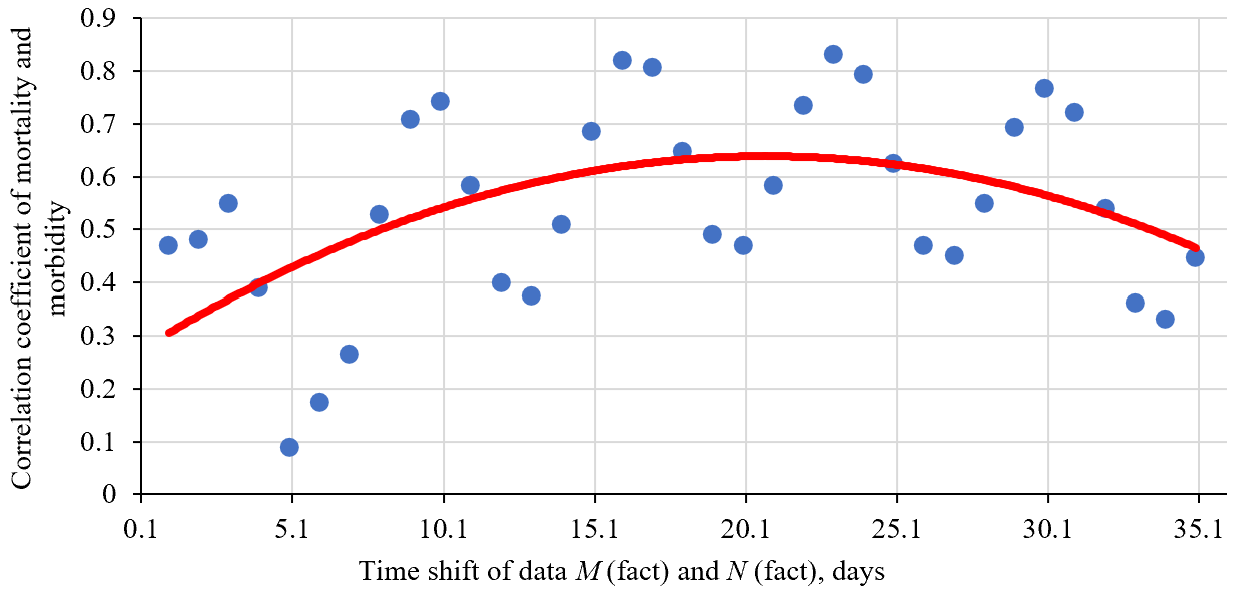
Fig. 6. Correlogram of mortality and morbidity depending on the shift parameter τ

Trend analysis shows the probability of death from COVID-19 on the 21st day after infection. In addition, the frequency of the risk of death is obvious. Trend-free variations of the risk of death are visualized in Fig. 7.

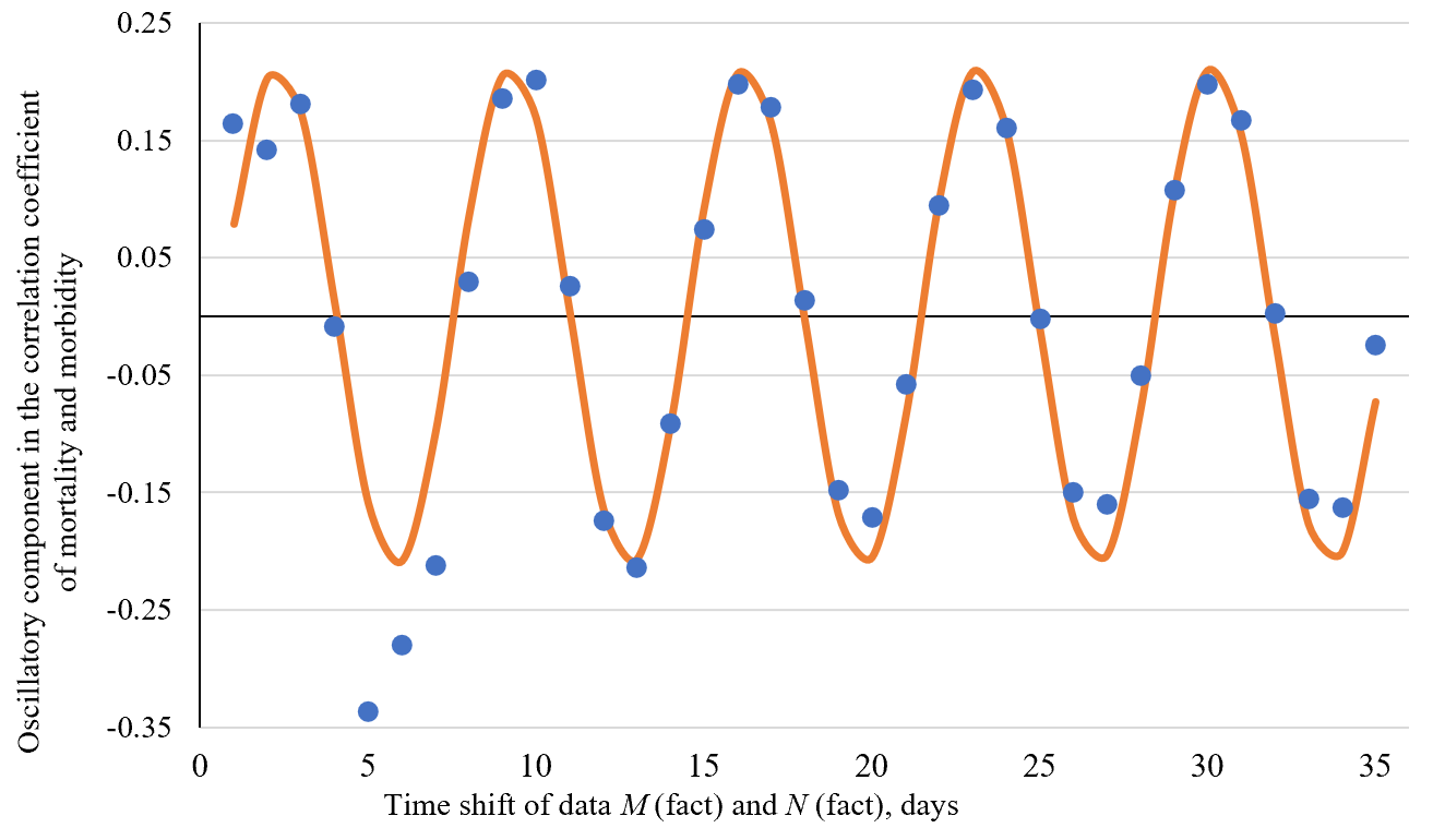
Fig. 7. Fast oscillation component in the correlogram of mortality and morbidity

According to Fig. 7, the risk of death in COVID-19 fluctuates around the above average value with a period of 7 days, which fully corresponds to the cyclical work of medical institutions around the world. The analytical dependence approximating the data in Fig. 7 has the form:

(23)

where  — the fast component of mortality.

Discussion and Conclusion. The main results of the work are listed below.

1. Models of morbidity and mortality in COVID-19 have been constructed and initialized.
2. It has been established that the spread of coronavirus infection is repeated three times a year.
3. Mortality is constant on average and contains two oscillation components. The frequency of the first one corresponds to the frequency of morbidity, and the frequency of the second one corresponds to the regulations of medical institutions.
4. Based on the observation interval from 12.02.2020 to 22.09.2021, it can be concluded that the scenario of the epidemic is close to pessimistic.
5. Random component in the morbidity and mortality models turned out to be at the level of seasonal fluctuations.

Statistical data that appeared in December 2021 showed that the known COVID-19 strains were practically replaced by a new one — omicron. Its contagiousness is 3/5 times higher; mortality is 3/5 times lower. This circumstance dictates the need to improve the proposed dynamic models of the epidemic, taking into account the virus-competitive effect. This is the objective of the following research by the team of authors.

The obtained results allow us not only to predict further dynamics of the pandemic, but also to formulate practically significant recommendations. For example, the following intervals are proposed as the optimal timing of anti-Covid vaccination by Sputnik V (annually): 05.02–15.02, 17.05–28.05, 24.09–5.10.

1 Сovid-19 coronavirus pandemic. International team of developers, researchers, and volunteers. Available from: https://www.worldometers.info/coronavirus/ (accessed 10.01.2023).

References

1. On the reliability of predictions on Covid-19 dynamics: A systematic and critical review of modelling techniques / E. G. Janyce, V. S. Kolawole, B. K. Gaеetan, G. K. Romain // Infectious Disease Modelling. — 2021. — V. 6. — P. 258–272. doi: 10.1016/j.idm.2020.12.008
2. Hermanowicz, S. W. Forecasting the Wuhan coronavirus (2019-nCov) epidemics using a simple (simplistic) model / S. W. Hermanowicz // MedRxiv. — 2020. — February. — 10 p. doi: 10.1101/2020.02.04.20020461
3. Lalmuanawma, S. Applications of machine learning and artificial intelligence for COVID-19 (SARS-CoV-2) pandemic: A review / S. Lalmuanawma, J. Hussain, L. Chhakchhuack // Chaos, Solitons & Fractals. — 2020. — V. 139, 110059. doi: 10.1016/j.chaos.2020.110059
4. Postniko, E. B. Estimation of COVID-19 dynamics «on a back-of-envelope»: Does the simplest SIR model provide quantitative parameters and predictions? / E. B. Postniko // Chaos, Solitons & Fractals. — 2020. — V. 135, 109841. doi: 10.1016/j.chaos.2020.109841
5. Брантон, С. Л. Анализ данных в науке и технике / С. Л. Брантон, Дж. Н. Куц // Москва : ДМК Пресс, 2021. — 574 с.
6. Виноградов, А. Ю. Численные методы решения жестких и нежестких краевых задач / А. Ю. Виноградов. — Москва : National Research, 2017. — 112 с.
7. Pugh, Ch. C. Real Mathematical Analysis. Second Edition / Ch. C. Pugh. — Cham : Springer, 2015. doi: 10.1007/978-3-319-17771-7
8. Maheshwari, A. Data Analytics Made Accessible / A. Maheshwari. — Bellevue : Kindle Edition, 2023. — 156 p.
9. Грибова, Е. З. Физический подход к анализу диффузии частиц / Е. З. Грибова, А. И. Саичев // Нижний Новогород : Нижегородский гос. ун-т им. Н. И. Лобачевского, 2012. — 232 с.
10. Егоров, А. И. Обыкновенные дифференциальные уравнения с приложениями / А. И. Егоров. — 2-е изд., исправ. — Москва : Физматлит, 2003. — 384 с.
11. Нестеров, Ю. Е. Методы выпуклой оптимизации / Ю. Е. Нестеров. — Москва : Московский центр непрерывного математического образования, 2010. — 281 с.
12. Ben-Tal, A. Lectures on Modern Convex Optimizatiоn Analysis, Alogorithms, and Engineering Applications / A. Ben-Tal, A. Nemirovski. — Philadelphia : SIAM, 2001. — 537 p.
13. Крянев, А. В. Математические методы обработки неопределенных данных / А. В. Крянев, Г. В. Лукин. — Москва : Физматлит, 2006. — 216 с.
About the Authors
N. N. AzimovaRussian Federation
Nataliya N. Azimova
1, Gagarin Sq.
Rostov-on-Don
M. V. Bedoidze
Russian Federation
Maria V. Bedoidze
S. N. Kholodova
Svetlana N. Kholodova
T. A. Mokina
Tatyana A. Mokina
Dz. Kh. Zairova
Dzhakhangul Kh. Zairova
A. S. Ermakov
Aleksandr S. Ermakov
Review
For citations:
Azimova N.N., Bedoidze M.V., Kholodova S.N., Mokina T.A., Zairova D.Kh., Ermakov A.S. Statistical Assessment of Biogenic Risk for the Human Population from New Viral Infections Based on COVID-19. Safety of Technogenic and Natural Systems. 2023;(1):4-15. https://doi.org/10.23947/2541-9129-2023-1-4-15