


Contents
Scroll to:
https://doi.org/10.23947/2541-9129-2025-9-2-146-157
EDN: TCVEAL
Scroll to:
Introduction. Estimation of the parameters of probability distribution laws using probability grids is widely used in practice, particularly in modern software systems. This approach is actively employed for statistical analysis, where the calculation results are presented as a probability graph. This allows for the assessment of the correspondence between a given data set and a proposed probability model, as well as the identification of outliers. In the context of probabilistic assessment of the loading of machine elements and structures, some authors suggest applying the Fisher–Tippett law. This law is characterized by a distribution function with three parameters and is oriented to the maximum. This provides flexibility in the description of statistical data and enables the estimation of the maximum value in the context of loading. Nevertheless, the existing literature has not sufficiently substantiated the graphical representation of calculation results and the method of parameter estimation, including the use of the probability grid method, which limits the practical application of the Fisher–Tippett law. Therefore, the aim of this study is to justify and develop a methodology for estimating parameters of the Fisher–Tippett law using the probability grid method.
Materials and Methods. The principles and theoretical foundations of constructing probability grids, the preliminary grouping of data, and a ranking method for estimating the empirical distribution were considered as the materials for the study. Analytical dependencies for constructing a probability grid and estimating the parameters of the Fisher–Tippett law were justified. The method of mathematical modeling and comparative analysis were employed. The Matlab 8.6 software package was utilized for modeling. The data were summarized in a tabular format and visualized in the form of graphs.
Results. The method of constructing a probabilistic graph and the method of graphical estimation of the parameters of the Fisher–Tippett law were justified and demonstrated by example. A graph of the empirical distribution function and a probability plot with a description of the locations were presented. A method for constructing a special scale for estimating the shape parameter centered on the origin was proposed. A comparative analysis of parameter estimates obtained using graphical and analytical methods was performed. Estimates of the scale, shape, and shift parameters were compared. The relative error in estimates using the probability grid method was not more than 2%. The indicator for the scale parameter was 1.83%; for the shape parameter was it 0.67%, and for the shift parameter it was 0.45%. Corresponding results of the analytical assessment were 4.4%, 9.33% and 2.13%. In this case, the error was higher, but it did not mean that the analytical method was less accurate.
Discussion and Conclusion. The adequacy of the proposed method of graphical estimation of the parameters of the Fisher–Tippett law by the probabilistic grid method has been demonstrated. This method can be applied, for example, within software packages or user applications. A special scale for graphically estimating the shape parameter can also be used to estimate the shape parameter of the Weibull law. The obtained analytical dependencies, the provisions of the methodology and the graphical materials can be used in the development of the corresponding national standard.
Kotesov A.A. Probability Grid Method for Fisher-Tippett Law. Safety of Technogenic and Natural Systems. 2025;(2):146-157. https://doi.org/10.23947/2541-9129-2025-9-2-146-157. EDN: TCVEAL
Introduction. Graphical representation of statistical analysis results in the form of probability graphs is widely used in modern software systems, particularly in the analysis of reliability or survival. This allows for the estimation of distribution law parameters and the identification of outliers1. Estimation of parameters using probability grids is used alongside other well-known methods and in some cases may be preferable. Probabilistic graphs are employed in the processing of resource test results2 and the creation of control maps in quality management systems3. The probability grid method enables a visual assessment of the correspondence between a data set and an assumed model for a random variable, as described in the works of M.A. Deryabin [1], S.A. Dobrotin [2], V.L. Shper [3], Ya.I. Bulanov [4], K.S. Ablazova [5], N.P. Velikanova [6], G.Sh. Khazanovich [7] and other modern scientists.
V.E. Kasyanov [8] and A.A. Kotesov [9] propose using one of the forms of generalized distribution of extreme values [10] with a certain type of parameterization, which they propose to call the Fisher–Tippett law, for probabilistic assessment of machine element and structure loading, but differs in that it focuses on maximum values. The Fisher–Tippett law is suitable for estimating reliability indicators in combination with the Weibull law, for example, when applying the load–strength failure model [11].
The graphical representation of the calculation results and the method used to estimate the parameters for the Fisher–Tippett law are not well justified. The scientific literature and regulatory and technical documents do not provide a specific method for estimating these parameters using a probability grid, which limits the practical application of this law. Therefore, the aim of this study is to develop and substantiate a methodology for estimating Fisher–Tippett law using the probability grid method.
Materials and Methods. Estimation of distribution parameters using probability graphs is based on grouping data by intervals and constructing an interval empirical distribution regardless of the assumed theoretical distribution. Therefore, such methods are often called nonparametric or rank-based. A probability grid is constructed for a specific probability distribution law in order to get a linear relationship between variables4. Plotting involves linear approximation of an array of empirical points on a probability grid. Therefore, this approach may be considered crude, but it is often used along with others. The probability grid method can be decisive in the case when other methods are untenable. For example, when estimating parameters using the maximum likelihood method, the likelihood function may contain several local maximas. In this case, parameter estimates can be very inaccurate [12].
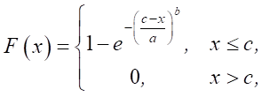
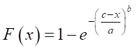
To justify the probability grid, we need to reduce the probability distribution function to a linear form. The Fisher–Tippett distribution function is defined by the following expression:
 (1)
(1)
where x — value of a random variable; a, b, c — scale, shape, and shift parameters of the distribution, respectively.
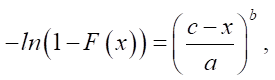
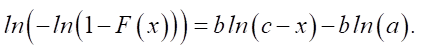
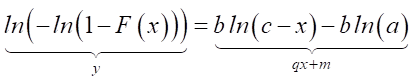
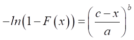
We transform distribution function (1) by taking the logarithm of both the left and right sides. Provided that c > х, we get:
 (2)
(2)
Obviously, expression (2) is a linear function of the form:
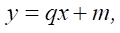 (3)
(3)
where х — function variable; q and m — constants.
Comparing (2) and (3), we get:
 .
.
Expression (2) differs from a similar sound to the Weibull distribution with three parameters in that only the right side is different:
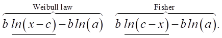
Therefore, to construct a probability graph of the Fisher–Tippett law, it is advisable to use the basic provisions of GOST 11.008 and GOST 50779.27. According to these standards, statistical data are plotted on a probability grid during graphical analysis, and then the distribution parameters are estimated. Let us note that the probability grid method is implemented both graphoanalytically and completely analytically. Therefore, to eliminate possible ambiguity, we will call the estimation of parameters using the probability grid method graphical, and the estimation by the maximum likelihood method analytical.
The left side of expression (2) allows us to determine the ordinate of the probability scale for estimating the scale parameter. Let us assume that с – х = а. By substituting this value in (2), we get:
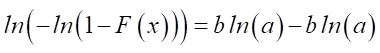 ,
,
 ,
,
 ,
,
 ,
,
 ,
,
 ,
,
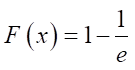 ,
,
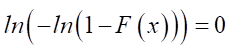
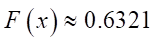 . (4)
. (4)
Result (4) allows us to conclude that the abscissa of the point approximating the line with zero ordinate will be an estimate of the scale parameter.
The decimal logarithm can be used along the abscissa axis of the probability graph. In this case, dependency (2) will take the form:
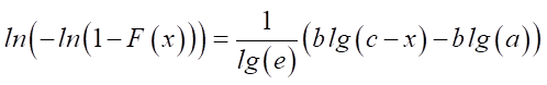 .
.
An important aspect of implementing the probability grid method is the initial processing of statistical data, specifically, obtaining an interval series of variations and estimating the empirical distribution function values. To obtain an empirical distribution function, a ranking method is typically used, which involves estimating the position of a distribution based on ordered data, considering the characteristics of the variation series (mean, median, mode, etc.). Therefore, various dependencies are used to determine the ordinates of points, including expressions for approximate estimation [13]. In this case, the choice will be determined by the amount of empirical data, the expected theoretical distribution, and the type of probability graph. This takes into account the need for an adequate description of the extreme members of the variation series [14].
It should be noted that some previous approaches to estimating the empirical distribution function have been criticized, and this may be the subject of a separate discussion [15].
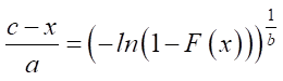
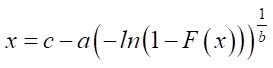
Results. The inverse function method is used to model a set of random data without a specific physical meaning, distributed according to the Fisher–Tippett law.
The inverse distribution function is obtained analytically from expression (1):
 ,
,
 ,
,
 ,
,
 ,
,
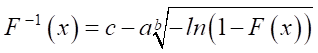 . (5)
. (5)
The simulation was conducted using the Matlab 8.6 software package, (Fig. 1), according to the specified parameters a, b, and c. The initial data used for the modeling are presented in Table 1.
Table 1
Initial data for modeling
|
Parameters of the Fisher–Tippett law |
Number of values |
||
|
a |
b |
c |
n |
|
100.00 |
3.00 |
250.00 |
100 |
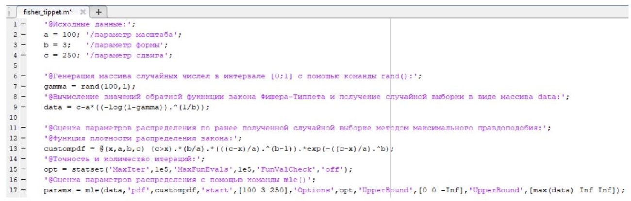
Fig. 1. Modeling a set of random data in Matlab 8.6
The simulation results in the form of a set of random data xi are presented in Table 2.
Table 2
A set of random data with no definite physical meaning
|
No. |
xi |
|||||||||
|
1 |
201.98 |
222.87 |
182.26 |
183.98 |
133.30 |
114.41 |
204.15 |
157.16 |
169.63 |
217.17 |
|
2 |
124.97 |
100.63 |
138.10 |
112.03 |
185.71 |
160.66 |
169.88 |
123.02 |
192.45 |
179.76 |
|
3 |
143.79 |
97.90 |
118.26 |
208.58 |
152.80 |
95.93 |
179.54 |
214.92 |
155.05 |
132.63 |
|
4 |
140.21 |
199.05 |
140.76 |
179.14 |
200.77 |
189.65 |
178.47 |
117.03 |
152.32 |
174.79 |
|
5 |
148.32 |
164.27 |
169.47 |
153.61 |
160.16 |
200.97 |
201.86 |
198.03 |
187.74 |
205.69 |
|
6 |
160.11 |
147.75 |
109.29 |
188.97 |
127.93 |
179.33 |
153.42 |
128.49 |
159.80 |
160.55 |
|
7 |
176.62 |
180.02 |
183.43 |
149.66 |
113.64 |
170.37 |
180.74 |
132.75 |
84.58 |
172.97 |
|
8 |
147.27 |
138.01 |
158.67 |
133.01 |
161.65 |
168.27 |
194.75 |
114.29 |
162.36 |
139.61 |
|
9 |
199.99 |
156.53 |
104.26 |
161.36 |
181.23 |
178.00 |
241.30 |
197.14 |
144.12 |
159.39 |
|
10 |
195.72 |
167.66 |
182.20 |
148.29 |
148.13 |
144.22 |
180.65 |
161.10 |
169.07 |
132.26 |
An analytical assessment of the scale, shape, and shift parameters has been conducted. The estimates are indicated respectively — a΄, b΄, c΄ (Table 3).
Table 3
Results of the analytical evaluation of the parameters
|
Estimates of the parameters of the Fisher–Tippett law |
||
|
a΄ |
b΄ |
c΄ |
|
104.40 |
3.28 |
255.32 |
The Fisher–Tippett law, unlike the Weibull law, has a restriction on the right and sets the maximum value for a random variable. Therefore, to obtain a series of variations, it is necessary to order the values in the dataset (sample) from maximum to minimum.
If the sample size is n ≤ 30, then it is not advisable to group the data by intervals. In such cases, each variant should be assigned a rank of j, and an approximation for the median position of these ranks can be used to estimate the values of the empirical distribution function [16]:
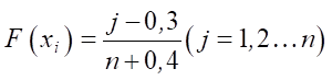 , (6)
, (6)
where xi — value of the sample variants ordered from maximum to minimum, corresponding to the j-th rank; j — ordinal number of the rank; n — sample size.
Otherwise, for n > 30 it is necessary to group the data by intervals in accordance with the absolute sample size. At the same time, it is recommended to take the number of interval k in the range of 7 ≤ k ≤ 40 depending on sample size n. To group the data, it is necessary to determine the boundaries of the interval by selecting the values X΄ ≤ xmin and X΄΄ ³ xmax, and divide the resulting interval [ X΄; X΄΄] into the intervals of equal length h:
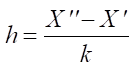 . (7)
. (7)
Then, an interval variation series should be obtained by determining the number of sample values ni, that fall within each interval. Each interval is described by abscissa Xi, which defines the position of the ordered data distribution.
For the middle position, the empirical distribution function is estimated using the expression:
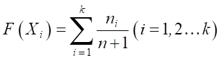 , (8)
, (8)
where Xi — middle of the i-th interval; ni — number of sample members that fell into the i-th interval; k — number of intervals; n — sample size.
As an example, the values of the empirical distribution function were grouped and calculated (Fig. 2) for the data set from Table 3.
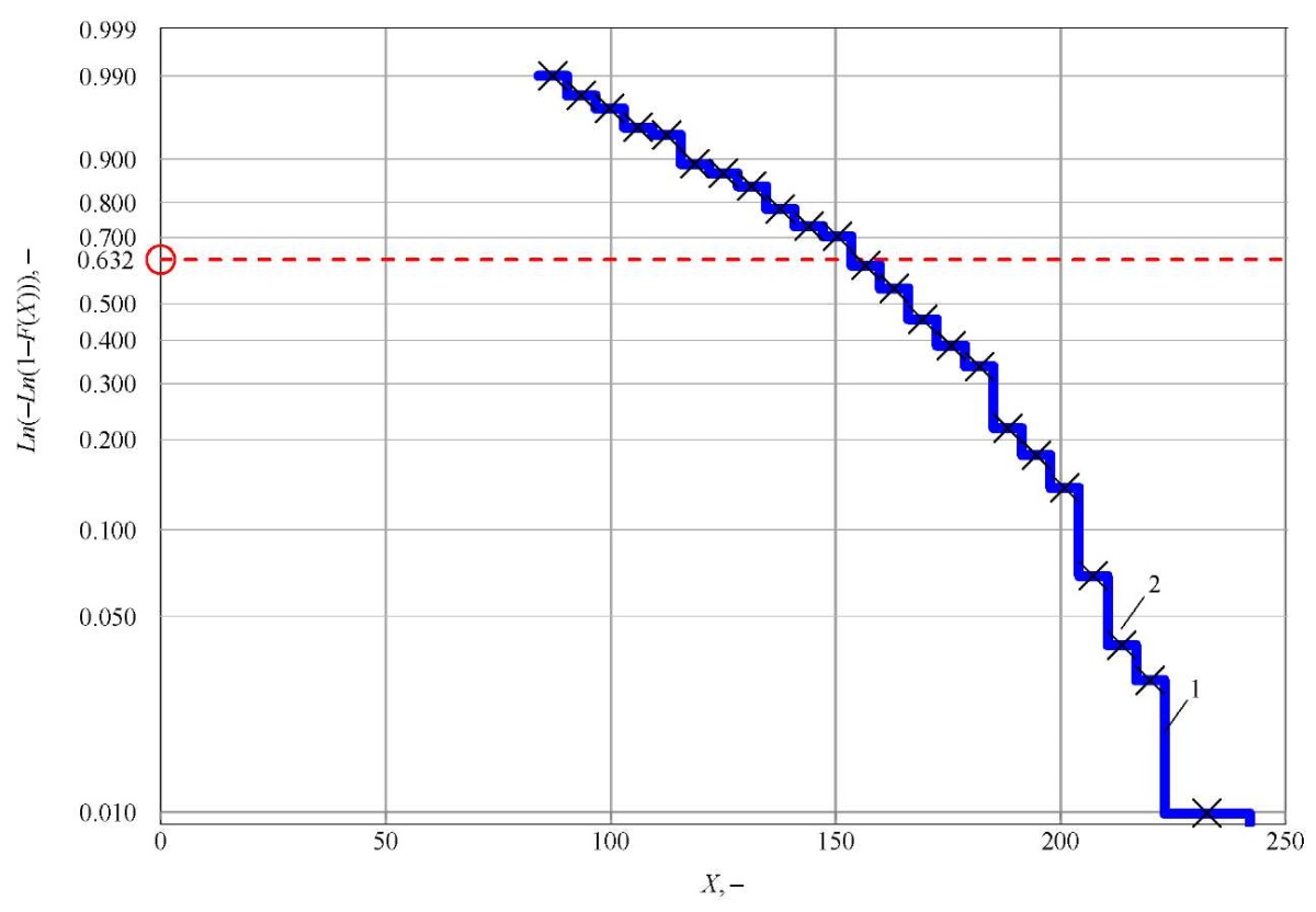
Fig. 2. Empirical distribution function: 1 — function; 2 — middle of the interval
Figure 2 shows the probability value along the ordinate axis; and the values of the dataset (sample) without a specific physical meaning are shown along the abscissa axis.
For data grouping, we assume k = 25, X΄ = 84, X΄΄ = 242 and determined value h = 6.32. One sample value falls into the first three intervals, so they are combined. The total number of intervals — k = 23. Table 4 provides the calculation results.
Table 4
Calculation results
|
i |
Rank interval |
ni |
Xi |
F(Хi) |
F(Хi)+F(Хi+1) |
Lg(Xi) |
Ln(–Ln(1–(F(Хi)+F(Хi+1)))) |
C'–Xi |
Lg(C'–Xi) |
|
|
beginning |
end |
|||||||||
|
1 |
2 |
3 |
4 |
5 |
6 |
7 |
8 |
9 |
10 |
11 |
|
1* |
223.04* |
242.00* |
1 |
232.52 |
0.0099 |
0.0099 |
2.3665 |
–4.6101 |
22.68 |
1.3555 |
|
2 |
216.72 |
223.04 |
2 |
219.88 |
0.0198 |
0.0297 |
2.3422 |
–3.5015 |
29.00 |
1.4623 |
|
3 |
210.40 |
216.72 |
1 |
213.56 |
0.0099 |
0.0396 |
2.3295 |
–3.2087 |
35.32 |
1.5480 |
|
4 |
204.08 |
210.40 |
3 |
207.24 |
0.0297 |
0.0693 |
2.3165 |
–2.6335 |
41.64 |
1.6195 |
|
5 |
197.76 |
204.08 |
7 |
200.92 |
0.0693 |
0.1386 |
2.3030 |
–1.9024 |
47.96 |
1.6808 |
|
6 |
191.44 |
197.76 |
4 |
194.60 |
0.0396 |
0.1782 |
2.2891 |
–1.6282 |
54.28 |
1.7346 |
|
7 |
185.12 |
191.44 |
4 |
188.28 |
0.0396 |
0.2178 |
2.2748 |
–1.4038 |
60.60 |
1.7824 |
|
8 |
178.80 |
185.12 |
12 |
181.96 |
0.1188 |
0.3366 |
2.2600 |
–0.8906 |
66.92 |
1.8255 |
|
9 |
172.48 |
178.80 |
5 |
175.64 |
0.0495 |
0.3861 |
2.2446 |
–0.7175 |
73.24 |
1.8647 |
|
10 |
166.16 |
172.48 |
7 |
169.32 |
0.0693 |
0.4554 |
2.2287 |
–0.4979 |
79.56 |
1.9007 |
|
11 |
159.84 |
166.16 |
9 |
163.00 |
0.0891 |
0.5446 |
2.2122 |
–0.2402 |
85.88 |
1.9339 |
|
12 |
153.52 |
159.84 |
7 |
156.68 |
0.0693 |
0.6139 |
2.1950 |
–0.0497 |
92.20 |
1.9647 |
|
13 |
147.20 |
153.52 |
9 |
150.36 |
0.0891 |
0.7030 |
2.1771 |
0.1939 |
98.52 |
1.9935 |
|
14 |
140.88 |
147.20 |
3 |
144.04 |
0.0297 |
0.7327 |
2.1585 |
0.2771 |
104.84 |
2.0205 |
|
15 |
134.56 |
140.88 |
5 |
137.72 |
0.0495 |
0.7822 |
2.1390 |
0.4214 |
111.16 |
2.0459 |
|
16 |
128.24 |
134.56 |
6 |
131.40 |
0.0594 |
0.8416 |
2.1186 |
0.6111 |
117.48 |
2.0699 |
|
17 |
121.92 |
128.24 |
3 |
125.08 |
0.0297 |
0.8713 |
2.0972 |
0.7179 |
123.80 |
2.0927 |
|
18 |
115.60 |
121.92 |
2 |
118.76 |
0.0198 |
0.8911 |
2.0747 |
0.7963 |
130.12 |
2.1143 |
|
19 |
109.28 |
115.60 |
5 |
112.44 |
0.0495 |
0.9406 |
2.0509 |
1.0379 |
136.44 |
2.1349 |
|
20 |
102.96 |
109.28 |
1 |
106.12 |
0.0099 |
0.9505 |
2.0258 |
1.1005 |
142.76 |
2.1546 |
|
21 |
96.64 |
102.96 |
2 |
99.80 |
0.0198 |
0.9703 |
1.9991 |
1.2575 |
149.08 |
2.1734 |
|
22 |
90.32 |
96.64 |
1 |
93.48 |
0.0099 |
0.9802 |
1.9707 |
–4.6101 |
155.40 |
2.1914 |
|
23 |
84.00 |
90.32 |
1 |
87.16 |
0.0099 |
0.9901 |
1.9403 |
–3.5015 |
161.72 |
2.2088 |
where * — Correction when combining intervals 1–3 into one interval [ 223,04; 242,00]
On the x-axis of the probability graph, we use a scale with decimal logarithms. The calculation results from columns 8 and 9 of Table 4 determine the coordinates of the points for plotting {Lg(Xi); Ln(–Ln(1–(F(Хi)+F(Хi+1))))}.
At the next stage, the shift parameter is evaluated. To do this, a smooth curve (rather than a straight line) (Fig. 3, pos. 2) should be drawn through the array of points (Fig. 3, pos. 1).
At the point where the straight line intersects the zero ordinate (Fig. 3, pos. 7), graphical estimation of scale parameter А΄ is made.
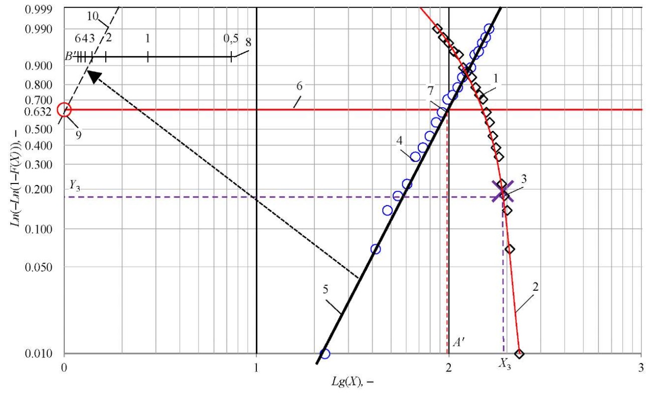
Fig. 3. Graphical estimation of the Fisher–Tippett law parameters: 1 — points with coordinates {Lg(Xi); Ln(–Ln(1–(F(Хi)+F(Хi+1)))}; 2 — line for estimating abscissa X3 along ordinate Y3; 3 — point with coordinates {Y3; X3}; 4 — points with coordinates {Lg(С΄–Xi); Ln(–Ln(1–(F(Хi)+F(Хi+1))))}; 5 — straight line approximating points 4; 6 — line for estimating the scale parameter; 7 — intersection point of lines 5 and 6, advising the estimation of scale parameter A΄; 8 — scale for estimating shape parameter B΄; 9 — point with coordinates {0; 0}; 10 — straight line drawn through point 9 parallel to straight line 5, to evaluate shape parameter B΄ on scale 8
Figure 3 shows the probability value along the ordinate axis, and the abscissa axis shows the values of a data set (sample) without a specific physical meaning.
The coordinates of the points of the extreme members of the variation series are denoted by {Х1; Y1} and {Х2; Y2}, and Y3 coordinate is estimated:
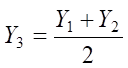 . (9)
. (9)
Using ordinate Y3 on the previously indicated curve, abscissa Х3 can be determined (Fig. 3, pos. 3). Then shift parameter С΄ is estimated:
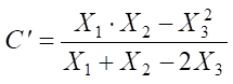 . (10)
In the example presented, the extreme terms of the variation series are the midpoints of intervals i = 1 and i = 23 with coordinates {Lg(X1); Ln(–Ln(1–(F(Х1)))} and {Lg(X23); Ln(–Ln(1–(F(Х22)+F(Х23)))}. Accordingly, Y1 = Ln(–Ln(1–(F(Х1))), Y2 = Ln(–Ln(1–(F(Х22)+F(Х23))), X1 = Lg(X1); X2 = Lg(X23). As a result, a graphical estimate of shift parameter С΄ = 248.88. We use it to adjust the abscissa of all points, determining values (С΄–Хi), and plot the points with the corresponding coordinates on the graph (Fig. 3, pos. 4). As you can see, after the correction, the points lined up “more evenly”, which allows us to draw a straight line through them (Fig. 3, pos. 5).
The estimate of the shape parameter corresponds to the angle of inclination of the approximating straight line (Fig. 3, pos. 5) to the abscissa axis. To graphically evaluate the parameter, you can use the coordinates of the points or a special scale (if available). When estimating the shape parameter by coordinates, it is necessary to express the values along the abscissa axis on the scale of the natural logarithm, i.e. use the value Ln(X) instead of Lg(X).
The considered example shows a scale for graphical evaluation of shape parameter B΄ (Fig. 3, pos. 8). To construct the scale, the coordinates of points {Lg(X); Ln(Y)} were calculated based on the set values of the shape parameter (Table 5). The scale is oriented to the reference point with coordinates {0; 0} (Fig. 3, pos. 9). To estimate the shape parameter, it is necessary to draw a straight line parallel to the approximating line through the reference point (Fig. 3, pos. 10).
Table 5
Building a scale for graphical evaluation of the shape parameter
|
B΄ |
0.5000 |
1.0000 |
2.0000 |
3.0000 |
4.0000 |
5.0000 |
6.0000 |
|
Ln(Y) |
1.0000 |
1.0000 |
1.0000 |
1.0000 |
1.0000 |
1.0000 |
1.0000 |
|
Ln(X) |
2.0000 |
1.0000 |
0.5000 |
0.3333 |
0.2500 |
0.2000 |
0.1667 |
|
Lg(X) |
0.8686 |
0.4343 |
0.2171 |
0.1448 |
0.1086 |
0.0869 |
0.0724 |
As a result of data processing, graphical estimates of the parameters of the Fisher–Tippett law were obtained (Table 6).
Table 6
Results of graphical parameter estimation
|
Estimates of the parameters of the Fisher–Tippett law |
||
|
A΄ |
B΄ |
С΄ |
|
98.17 |
2.98 |
248.87 |
After evaluating the parameters, we need to perform a check using inverse function (5) with the specified probability values:
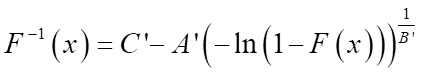 . (11)
By calculating the values of inverse distribution function (11) and connecting the resulting points on the graph, you can visually assess the quality of the model. As you can see, the graph of the inverse function (Fig. 4) smoothly describes the array of initial points (Fig. 4, pos. 1 and 2). This suggests that the model is able to accurately describe the data, and the parameter estimation has been performed correctly.
Fig. 4. Checking the model after graphical evaluation of the parameters
1 — starting points with coordinates {Lg(Xi); Ln(–Ln(1–(F(Хi)+F(Хi+1)))};
2 — graph of inverse distribution function F–1(x) with parameters A΄, B΄, С΄
Figure 4 shows the probability value along the ordinate axis, and the abscissa axis shows the values of the data set (sample) without a specific physical meaning.
The results of the verification calculations are presented in Table 7.
Table 7
The results of the model's testing
|
F(x) |
F–1(x) |
Lg(F–1(x)) |
Ln(–Ln(1–(F(x)) |
|
0.0010 |
239.1548 |
2.3787 |
–6.9073 |
|
0.0050 |
232.2033 |
2.3576 |
–5.2958 |
|
0.0100 |
227.8309 |
2.3068 |
–4.6001 |
|
0.0500 |
212.5564 |
2.2775 |
–2.9702 |
|
0.1000 |
202.6589 |
2.2537 |
–2.2504 |
|
0.2000 |
189.4586 |
2.2317 |
–1.4999 |
|
0.3000 |
179.3564 |
2.2096 |
–1.0309 |
|
0.4000 |
170.4725 |
2.1862 |
–0.6717 |
|
0.5000 |
162.0373 |
2.1596 |
–0.3665 |
|
0.6000 |
153.5320 |
2.1263 |
–0.0874 |
|
0.7000 |
144.4053 |
2.0758 |
0.1856 |
|
0.8000 |
133.7435 |
2.0299 |
0.4759 |
|
0.9000 |
119.0766 |
1.9303 |
0.8340 |
|
0.9900 |
85.1730 |
1.8882 |
1.5272 |
|
0.9990 |
61.3715 |
1.7880 |
1.9326 |
As it can be seen, the graphical and analytical estimates of the parameters are close to the parameters set during the modeling of the dataset (a, b, c).
It is not entirely correct to compare the estimates obtained with respect to the specified parameters, however, such a comparison is justified if the specified parameters are taken as the true parameters of the general population, and the set of random data хi is considered a representative sample. A comparative analysis of graphical and analytical estimates is presented in Table 8.
Table 8
Comparison of graphical and analytical estimates of parameters
|
Indicator |
Scale parameter |
Value |
δ, % |
Shape parameter |
Value |
δ, % |
Shift parameter |
Value |
δ, % |
|
Preset parameters |
a |
100.00 |
– |
b |
3.00 |
– |
c |
250.00 |
– |
|
Analytical estimation of parameters |
a΄ |
104.40 |
4.40 |
b΄ |
3.28 |
9.33 |
c΄ |
255.32 |
2.13 |
|
Graphical estimation of parameters |
A΄ |
98.17 |
1.83 |
B΄ |
2.98 |
0.67 |
С΄ |
248.87 |
0.45 |
Comparative analysis has shown that the relative error of graphical estimates does not exceed 2% (δ < 2%). The error of the analytical estimates in this example turned out to be higher, but this does not mean that the analytical method is less accurate.
Discussion and Conclusion. The presented probability grid method for the Fisher–Tippett law is adequate and suitable for practical application. For example, it can be used in software packages or when creating custom applications for graphical representation of statistical analysis results. It opens up the possibility to perform model fitting together with other known methods, even if they are untenable. The proposed method of constructing a scale for graphically estimating the shape parameter can be used to evaluate the shape parameter of the Weibull's law. The obtained analytical dependencies, the provisions of the methodology and the graphic material can be useful in the development of an appropriate national standard.
1. GOST R ISO 16269–4–2017. Statistical methods. Statistical data presentation. Part 4. Detection and treatment of outliers. Electronic Fund of Legal and Regulatory and Technical Documents (In Russ.) URL: https://docs.cntd.ru/document/1200146680 (accessed: 15.01.2025).
2. GOST R 50779.27–2017. Statistical methods. Weibull distribution. Data analysis. Electronic Fund of Legal and Regulatory and Technical Documents. (In Russ.) URL: https://docs.cntd.ru/document/1200146523 (accessed: 15.01.2025).
3. GOST ISO 7870–1–2022. Statistical methods. Control charts. Part 1. General guidelines. Electronic Fund of Legal and Regulatory and Technical Documents. (In Russ.) URL: https://docs.cntd.ru/document/1200192703 (accessed: 15.01.2025).
4. GOST 11.008–75. Applied statisticas. Graphic methods of data processing. Use of probability papers. (In Russ.) URL: https://meganorm.ru/Data2/1/4294753/4294753131.pdf (accessed: 15.01.2025).
1. Deryabin M, Bavykin O, Dyakov D. Application of the Probabilistic Paper Method to Determine the Law of Distribution of Measurement Results. In: Proceedings of II International Scientific and Practical Conference “Modern Trends in the Development of Science and Education: Theory and Practice”. Moscow: Institute of System Technologies; 2018. P. 67–72. (In Russ.)
2. Dobrotin SA, Kosyreva ON. Assessing the Presence of Outlier in Retention Time Data from Chromatographic Analysis. In: Proceedings of International Scientific and Practical Conference Science and Technology Research — 2024. Petrozavodsk: New Science; 2024. P. 11–22. URL: https://sciencen.org/assets/Kontent/Konferencii/Arhivkonferencij/KOF-971.pdf?ysclid=m6huh354xe556269601 (In Russ.) (accessed: 15.01.2025).
3. Shper VL. Quality Tools and More! Part 5. Analysis of the Distribution Law Using Probability Grids .Methods of Quality Management. 2021;8:54–60. (In Russ.)
4. Bulanov YaI, Moshkalo NG, Kurdenkova AV, Shustov YuS, Malyuga DК. Establishment of Empirical Laws of Distribution for Key Quality Indicators of Para-Aramid Fabrics for Armored Packages with Anti-Cut and Anti-Punch Properties. The News of Higher Educational Institutions. Technology of Light Industry. 2023;59(1):106–109. (In Russ.) https://doi.org/10.46418/0021-3489_2023_59_01_20
5. Ablazova KS. Control Charts that Determine the Stability of the Technological Process and Their Applications. Problems of Computational and Applied Mathematics. 2023;3(49):124–134. (In Russ.)
6. Velikanova NP, Velikanov PG. Changing the Heat Resistance of the Turbine Blades Material with Taking into Account the Influence of Operational Life. Ecological Bulletin of Research Centers of the Black Sea Economic Cooperation. 2023;20(2):42–48. (In Russ.) https://doi.org/10.31429/vestnik-20-2-42-48
7. Khazanovich GSh, Apryshkin DS. Assessment of the Influence of Internal Factors on the Indicators of Passenger Elevator Units Utilization Based on the Results of Regular Monitoring. Safety of Technogenic and Natural Systems. 2023;7(3):34–43. https://doi.org/10.23947/2541-9129-2023-7-3-34-43
8. Kasyanov VE, Demchenko DB, Kosenko EE, Teplyakovа SV. Method of Machine Reliability Optimization Using Integral Indicator. Safety of Technogenic and Natural Systems. 2020;1:23–31. https://doi.org/10.23947/2541-9129-2020-1-23-31
9. Kotesov AA. Fisher-Tippet Law Truncated Form for Loading Modeling of Machinery Structures. Safety of Technogenic and Natural Systems. 2024;8(4):39–46. https://doi.org/10.23947/2541-9129-2024-8-4-39-46
10. Fisher RA, Tippet LHC. Limiting Forms of the Frequency Distribution of the Longest of Smallest Member of Sample. Mathematical Proceedings of the Cambridge Philosophical Society. 1928;24(2),180–190. https://doi.org/10.1017/S0305004100015681
11. Kolesov AA, Kotesova AA. Comprehensive Correction Strength and Loads Characteristics Sample Distributions Parameters at Machinery Engineering Objects Reliability Optimization. News of the Tula State University. Technical Sciences. 2023;8:699–708. (In Russ.) https://doi.org/10.24412/2071-6168-2023-8-699-700
12. Lawless JF. Statistical Models and Methods for Lifetime Data, 2nd ed. Hoboken: Wiley; 2011. 664 p.
13. Ross R. Graphical Methods for Plotting and Evaluating Weibull Distributed Data. In: Proc. of 1994 4th International Conference on Properties and Applications of Dielectric Materials (ICPADM). Brisbane, QLD, Australia; 1994. P. 250–253 http://doi.org/10.1109/ICPADM.1994.413986
14. Hyndman RJ, Yanan Fan. Sample Quantiles in Statistical Packages. The American Statistician. 1996;50(4):361–365. http://doi.org/10.1080/00031305.1996.10473566
15. Makkonen L, Pajari M, Tikanmäki M. Discussion on “Plotting Positions for Fitting Distributions and Extreme Value Analysis”. Canadian Journal of Civil Engineering. 2013;40(9):927–929. https://doi.org/10.1139/cjce-2013-0227
16. Benard A, Bos-Levenbach EC. Het uitzetten van waarnemingen op waarschijnlijkheids-papier. Statistica Neerlandica. 1953;7(3):163–173. https://www.sci-hub.ru/10.1111/j.14679574.1953.tb00821.x?ysclid=m6hw1ukl7k731787987
Anatoly A. Kotesov, Cand.Sci. (Eng.), Associate Professor of the Department of Transport Systems and Logistics
1, Gagarin Sq., Rostov-on-Don, 344003
Kotesov A.A. Probability Grid Method for Fisher-Tippett Law. Safety of Technogenic and Natural Systems. 2025;(2):146-157. https://doi.org/10.23947/2541-9129-2025-9-2-146-157. EDN: TCVEAL


Safety of Technogenic and Natural Systems
eISSN 2541-9129
Contact with: Publisher / Editorial Office of the Journal
Publisher: Don State Technical University - DSTU, Rostov-on-Don, Russia - https://donstu.ru/en/
Editor-in-Chief: Meskhi Besarion Chokhoevich, Doctor of Technical Sciences, Professor (Rostov-on-Don, Russia)
Don State Technical University
1, Gagarin Sq., Rostov-on-Don, 344003, Russia
tel.: +7 (863) 2738-372, e-mail: btps@donstu.ru
1, Gagarin Square, Rostov-on-Don, 344003, Russian Federation, Don State Technical University
Processing of personal data


