


Contents
Scroll to:
https://doi.org/10.23947/2541-9129-2025-9-4-305-318
EDN: OBWTCN
Scroll to:
Introduction. Ignoring the systemic nature of a reservoir can lead to ineffective and damaging management decisions. However, the study of such objects often focuses on individual factors. The predictive potential of graph models is limited by a lack of expert information and outdated databases of indicators. This work aims to address these issues by evaluating the effectiveness of measures to improve the condition of the Tsimlyansk Reservoir. The solution is based on the author's graph model that takes into account the interaction of anthropogenic and biotic characteristics of the object.
Materials and Methods. The literature sources and information on hydrobiochemistry and species composition of fish were analyzed. A model was created that took into account 20 factors related to the state of the Tsimlyansk Reservoir. A hydrobiological analysis allowed us to create graph G(V, E, Y). V — set of vertices, vk ∊ V, k = 1̅, ̅2̅0. E — set of oriented edges ek = (vi, vj) in the form of ordered pairs of length 2, i ≠ j. Y — mapping, Y : V → V. A weight matrix was created based on an integral assessment of each factor by experts. The weighting coefficients (±0.5–±1) were calculated using information from hydrobiological and chemical databases.
Results. We investigated how the removal of zebra mussels would affect the facility during a single cleaning (scenario 1) and a three-year cleaning (scenario 2). We visualized the dynamics of pulses for the state of the water (v15) and changes in the concentration of biological substances (v18). In the first scenario, for the first factor, the maximum pulse (0.5) was fixed from the third year of exposure; the minimum (0) was during the first year. For the second factor, the pulse increased from a minimum (–0.5) to a maximum (0.25) over the third year. In the second scenario, both factors did not change in the first year. Then the pulse for v15 increased (to 0.75), v18 fell in the second year to –0.5, and then increased to –0.25.
Bream reproduction with v5 feeding was evaluated for a year (scenario 3) and five years (scenario 4). The state of spawning fish v1, replenishment of juveniles v2, fishing v7, and eutrophication v14 were taken into account. v2, v7, and v14 pulses remained zero for two years. Then v2 and v7 grew to one, and in the fourth year they fell to zero. The eutrophication pulse dropped to –1, and returned to zero by the end of the fourth year. With a five-year feeding, v1 pulse dropped to –1 in the first year, v14 — in the third, and its value did not change, and v1 returned to 0 in the fifth year of modeling. The pulse for v2 and v7 grew from zero to one in three years.
Discussion. Annual cleaning of a reservoir from zebra mussel was more effective for improving the water condition and less effective for the concentration of nutrients. One-time feeding would increase the number of juveniles and fishing. Eutrophication would decrease, but there would be no sustainable results. Annual feeding would increase the number of juveniles, reduce eutrophication and lead to the development of fishing.
Conclusion. The proposed solution makes it possible to predict potential benefits or harm of anthropogenic activities on the reservoir. The model can be improved by fine-tuning the weighting coefficients, taking into account non-linear and threshold effects as well as other indicators.
Kuznetsova I.Yu., Nikitina A.N. Study of Artificial Reservoir's Bioproductivity Based on a Graph Model of Natural and Anthropogenic Factor Interaction. Safety of Technogenic and Natural Systems. 2025;9(4):305-318. https://doi.org/10.23947/2541-9129-2025-9-4-305-318. EDN: OBWTCN
Introduction. A hydrobiological study of a reservoir allows us to assess the ecological state of aquatic ecosystems and develop measures for their conservation and restoration. Reservoirs are important environmental facilities. They provide water supply to the population, industry, and agriculture. However, the quality of the aquatic environment is deteriorating due to anthropogenic influence. Urban and agricultural runoff and waste change the temperature of reservoirs, disrupt the natural food supply, and promote the growth of harmful plants and animals [1]. All this leads to a decrease in the bioproductivity of reservoirs, i.e. generates environmental and economic risks.
The Tsimlyansk Reservoir is a source of drinking water for millions of residents of the Rostov and Volgograd Regions. It is important to monitor changes in the hydrobiological indicators of the reservoir and to develop methods for the protection and restoration of the ecosystem [2].
The creation of effective strategies for the conservation and restoration of the ecosystem of a reservoir requires a deep understanding of the mechanisms of interaction between its anthropogenic and biotic characteristics.
Russian and foreign scientists have studied the factors that affect the productivity of artificial reservoirs, but many challenges remain unsolved. Additionally, an integrated approach to addressing environmental quality issues in these reservoirs has not become the standard.
The key anthropogenic factor affecting the biotic health of a reservoir is water level [3]. Success of spawning [4], survival rate of juveniles, availability of feed biotopes, and wintering [5] depends on it. Therefore, drawdown (lowering) of the water level in a reservoir can be dangerous. Due to this, roe of phytophilic fish (carp, bream, crucian carp, roach) die during spawning. However, after spawning, lower water levels provide good warming for shallow waters, thus improving feeding conditions for juveniles.
Both natural and anthropogenic factors can be the causes of eutrophication. On the one hand, it increases the productivity of zooplankton (feed for juveniles), on the other hand, it can cause toxic blooms, as well as hypoxia and benthic death (feed for bottom-dwelling fish) [6].
Source [7] demonstrates the impact of toxic substances on water quality and productivity in reservoirs. Book [8] presents a comprehensive analysis of the impact of fishing, overfishing and the choice of fishing gear on fish populations. In [9], the causes and consequences of the introduction of new species of shellfish and fish into freshwater reservoirs are analyzed. It has been shown that alien species change biogeochemical cycles and the biotic composition of ecosystems. Invasive species can compete with native species or become a new target. Source [10] summarizes the results of long-term research by scientists from the Zoological Institute of the Russian Academy of Sciences, exploring the causes and mechanisms behind species dispersal and biodiversity in terrestrial and aquatic ecosystems, as well as the influence of alien species. Authors [11] evaluate the risks of biological invasions in marine coastal ecosystems through the example of Primorsky Krai. Article [12] explores the biodiversity of the Tsimlyansk Reservoir, identifies new species of zooplankton, and defines the zones of their settlement in the reservoir.
Let us specify the biotic factors essential for the productivity of water areas:
So, there is open access literature on certain conditions that affect the productivity of reservoirs. However, the interaction of these factors and their cumulative impact on biodiversity and commercial fish populations have not been sufficiently studied. Ecosystems of reservoirs are characterized by high dynamics of transformations, spatial heterogeneity and nonlinear relationships between various factors [14]. In recent decades, network models have become widespread, allowing for the analysis of dynamic relationships between individual species and environmental parameters.
Graph models allow you to identify key nodes, simulate impact scenarios, and quantify strength and direction of connections. These solutions show the structure of interactions, with nodes representing factors and edges representing connections. One example of using graph models in ecology is the description of trophic networks from several intertwining food chains. This approach is needed to analyze sustainability and identify key species [15]. It is also widely used in modeling habitat connectivity, describing migration processes [16], and modeling the impact of a specific species or factor on an ecosystem [17]. In [18], a graph model of the interaction between anthropogenic and biotic factors allowed researchers to evaluate the effectiveness of artificial population restoration for the Caspian Sea, which had been subjected to excessive commercial fishing.
Thus, the study of the graph model of the interaction between anthropogenic and biotic factors offers the potential for high-quality solutions to practical problems:
In addition, thanks to the proposed approach, it is possible to scientifically justify recommendations for the protection of unique reservoir ecosystems. The graph model clearly reflects the complex structure of cause-and-effect relationships within the ecosystem of the reservoir, making it possible to quantify the strength and direction of influence of various factors and perform a scenario analysis of the consequences of various changes in the ecosystem. The aim of this research is to construct a graph model of the interaction between anthropogenic and biotic factors in the Tsimlyansk Reservoir, as well as evaluate the effectiveness of different measures to improve its ecological state.
Materials and Methods. When determining materials and methods, we considered, in particular, the characteristics of the research object. The Tsimlyansk Reservoir, located on the Don River in the Rostov and Volgograd Regions, is one of the largest and most significant artificial reservoirs in southern Russia.
The Tsimlyansk Reservoir belongs to the type of flat run of the river reservoirs, with a highly developed coastline.
Its characteristics are:
Significant seasonal and long-term fluctuations in water levels are determined by the operation of water intake facilities, hydroelectric power plants, and climatic conditions such as snowmelt, precipitation, and evaporation. The weak spring flood can be explained by overregulation of the Don upstream the reservoir. In recent years, there has been a significant decrease in water intake1.
Winter is characterized by stable ice cover, while summer sees clear temperature stratification. Due to this, oxygen deficiency occurs and hypolimnion is formed, especially in deep-water areas.
The Tsimlyansk Reservoir was built in 1952 and completely filled in 1953. The facility is used for fishing, water supply to the population in the Rostov and Volgograd Regions, irrigation of agricultural land and electricity generation. Additionally, the reservoir ensures the operation of the Volga-Don Shipping Channel.
In recent decades, there has been a change in the hydrobiological regime of the reservoir under the influence of natural and anthropogenic factors.
Long-lasting high levels of biogenic elements (nitrogen and phosphorus compounds) with wastewater and agricultural runoff lead to a deterioration of the oxygen regime and the formation of dead zones. In such conditions, toxic species of cyanobacteria develop, phytoplankton grow (“blooming” of water) [19]. Other features of the reservoir:
A large mass of vegetation in shallow water negatively affects natural reproduction of commercial fish species [20].
Intensive long-term operations, powerful anthropogenic impacts, and natural aging processes have led to significant transformations in the ecosystem and a deterioration of the hydrobiological conditions of the reservoir.
In addition, the productivity of the reservoir is significantly reduced for at least two reasons:
Monitoring and assessment of the system's condition, identification of key problems and forecasting their development are critically important for developing strategies for sustainable reservoir management3 and preventing its further degradation [21].
The choice of the graph model and its components is explained below.
The analysis of an artificial reservoir is a complex and time-consuming process. It requires taking into account various factors that influence the condition of the reservoir:
Models describing hydrobiological processes in a reservoir can be divided into several classes.
Thus, the known models are either too simplified and unsuitable for accounting for complex interactions (as statistical), or excessively complex to construct and resource-intensive for operational use (dynamic, agent-oriented and hydrodynamic), or do not provide quantitative forecasts (conceptual).
Graph models are a relatively simple and flexible tool capable of integrating heterogeneous data (physical, chemical, biological, anthropogenic) and visualizing the structure of their interactions for analyzing and predicting the state of fish resources.
The analysis of ichthyology models made it possible to study in detail the factors determining the production and distraction processes in the reservoir. For example, article [18] considers a graph system of the influence of anthropogenic and biotic factors on reservoir productivity. The author of this work identified twelve factors as the vertices of the graph, which largely determined the dynamics of the sturgeon population. In [25], the role of fishing in population dynamics was shown, taking into account the age and sex of individuals. In [26], in addition to fishing, seasonal changes in the habitat of Theragra chalcogramma pollock were taken into account.
The disadvantages of the considered models include the lack of consideration of spatially heterogeneous hydrodynamic processes. In addition, many models ignore an important condition for the reproduction of commercial fish — the mechanism of external hormonal regulation of phyto- and zooplankton.
Based on the analysis of hydrobiological state of the Tsimlyansk Reservoir and some mathematical models of population dynamics, the following factors were taken into account when constructing the graph model: v1 — state of the spawning part of the fish population; v2 — annual replenishment of juveniles; v3 — natural (compensatory) loss of generation; v4 — favorable puberty conditions; v5 — specific efficiency of natural reproduction (feeding); v6 — scale of artificial release; v7 — level of commercial exploitation of fish biological resources; v8 — biomass of the dominant type of feed benthos; v9 — roe oxygen supply in the spawning area; v10 — transgression of the level of the Tsimlyansk Reservoir; v11 — number of the main natural enemies of juveniles; v12 — available length of spawning migration routes; v13 — overgrowth of zebra mussels (Dreissena polymorpha); v14 — eutrophication; v15 — state of the Tsimlyansk reservoir waters; v16 — changes in bream biomass; v17 — changes in the concentration of phyto- and zooplankton; v18 — changes in the concentration of biogenic substances (nitrogen, phosphorus, silicon compounds); v19 — influence of abiotic factors (salinity, temperature); v20 — anthropogenic impact (cleaning of the reservoir bottom from an invasive species — zebra mussels).
Based on the analysis of the hydrobiological state of the Tsimlyansk reservoir, graph G(V, E, Y) was obtained. Here:
The resulting graph model (cognitive map) of the bioproductivity of the Tsimlyansk Reservoir is presented in Figure 1. In this graph, the dotted lines represent positive effects, and the solid lines represent negative ones. A single arrow indicates a weak impact, while a double arrow indicates a strong impact.
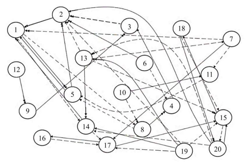
Fig. 1. Graph model of the Tsimlyansk Reservoir bioproductivity
The weight matrix of the graph model was generated based on an integral assessment of expert opinions, considering the significance of each factor's influence. Experts included specialists in fields such as hydrobiology, aquatic ecosystem ecology, ichthyology, mathematical modeling, computational mathematics, programming, etc. When calculating the weighting coefficients of the matrix, a continuously updated information base on hydrobiology and chemistry was utilized. This information was created by the researchers over many years of fieldwork.
In addition, the authors analyzed literary sources, information obtained from remote sensing of the Earth, as well as data on:
Further, when analyzing the influence of certain factors on the Tsimlyansk Reservoir productivity, the weighting coefficient for a weak impact (single arrow) will be ±0.5, and for a strong impact (double arrow) — ±1.
Results. A Python software package has been developed to numerically implement the graph-based productivity model of the Tsimlyansk Reservoir. This package allows users to work with both individual subgraphs and a complete cognitive map of the Tsimlyansk Reservoir bioproductivity (Fig. 1). This enables a more accurate description of the processes that affect the ecosystem of the reservoir.
The main steps of the algorithm for implementing the graph-based productivity model of the Tsimlyansk Reservoir are outlined below.
Step 1. Determining the set of graph vertices by selecting the vertices of the graph model under consideration (Fig. 1). Setting modeling time interval N (in years) and the time layer number n = 1.
Step 2. Assignment of the initial vector of vertex weights (factors) for the constructed graph model:
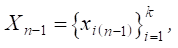
where k — number of vertices (factors) considered.
Step 3. Setting the relationship matrix (weight of graph edges) Un, obtained on the basis of expert opinions, for current time layer  . For mild exposure — ±0.5, for strong — ±1, without exposure — 0
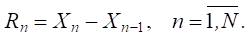
Step 4. Setting the vector of external pulses  for current time layer n.
Step 5. Calculation of momentum vector Rn for current time layer n [18]:
 (1)
(1)
Step 6. Recalculation of the vertex weight vector (factors) for current time layer n [18]:
 (2)
(2)
Step 7. If n < N, then go to step 5. Otherwise, the work will be completed and the graph will be build.
Taking into account expression (2), formula (1) can be represented as follows:
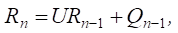
or
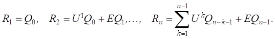 (3)
(3)
We believe that there are several possible scenarios for increasing the productivity of the Tsimlyansk reservoir. In the first scenario, we consider removing the invasive species — zebra mussels — from the reservoir through one-time cleaning measures (only in the first year).
Scenario 1. Thus, the anthropogenic impact was the cleaning of the bottom of the Tsimlyansk Reservoir from the zebra mussels in the first year.
In the graph model for this scenario, we included the following factors (vertices) from the full model (Fig. 1): v15 — state of the Tsimlyansk reservoir waters; v18 — changes in the concentration of biogenic substances (nitrogen, phosphorus, silicon compounds); v20 — anthropogenic impact (cleaning of the reservoir bottom from an invasive species — zebra mussels).
Figure 2 shows a graph model (a subgraph of the graph from Figure 1) of this scenario. The color highlights the factor that was affected by a positive external pulse.
The situation was modeled over a period of three years.
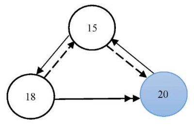
Fig. 2. Graph model for Scenario 1
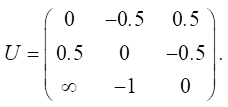
Let us define relationship matrix U for the graph model (Fig. 2):
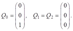
Let us set the vector of external pulses. Cleaning occurred only in the first year, so we set a positive pulse +1 at the beginning of v20 for Q0. For the remaining years, we do not apply any external pulses:
Let us calculate Rn pulses:
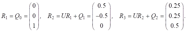
Figure 3 shows the results of changes in Rn pulses for water status factors v15 and changes in the concentration of nutrients (v18).
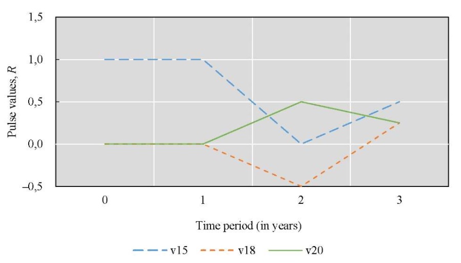
Fig. 3. Simulation results for Scenario 1
Scenario 2. Let us consider the anthropogenic impact — the annual cleaning of the bottom of the Tsimlyansk Reservoir from zebra mussels for three years.
The cognitive map of this scenario is also described in Figure 3. Relationship matrix U is as in Scenario 1.
Let us set the vector of external pulses +1 at vertex v20 in each year of the simulation:
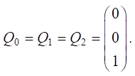
Let us calculate Rn pulses:
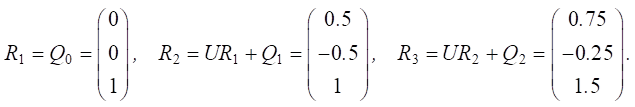
Figure 4 shows the results of changes in Rn pulses for the three factors considered over time.
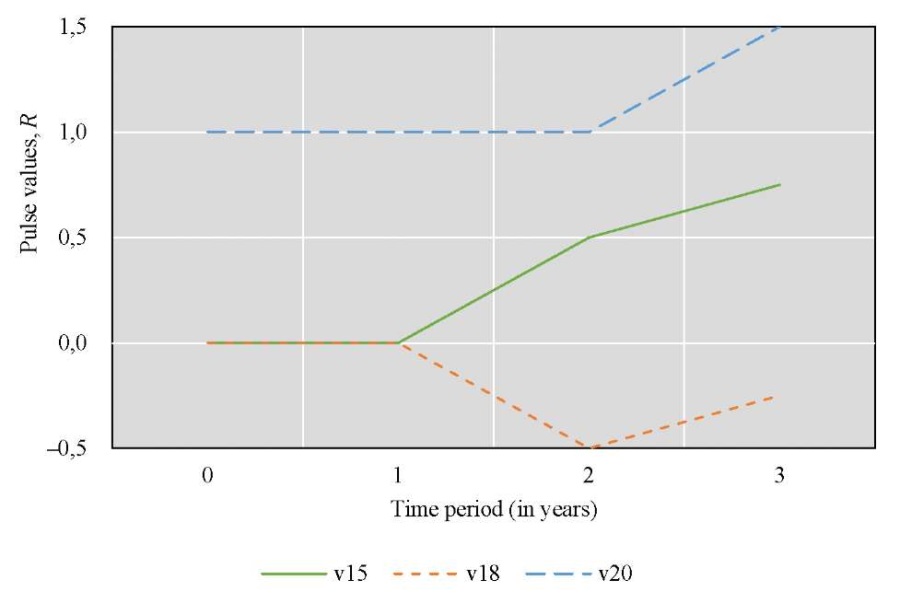
Fig. 4. Simulation results for Scenario 2
Let us consider two scenarios of anthropogenic impact on the specific efficiency of natural reproduction of commercial fish (bream) in the Tsimlyansk Reservoir — for a year and for five years
Scenario 3. Let us imagine the specific efficiency of natural bream reproduction in the Tsimlyansk Reservoir, when using feed additives for their nutrition during the first year.
The graph model included the following factors (vertices): v1 — state of the spawning part of the fish population; v2 — annual replenishment of juveniles; v5 — specific efficiency of natural reproduction (feeding); v7 — level of commercial exploitation of fish biological resources; v14 — eutrophication.
Figure 5 shows a cognitive map of this scenario.
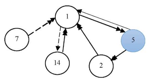
Fig. 5. Graph model for Scenario 3
The dynamics of the situation over a five-year period are modeled.
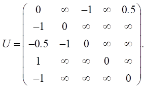
Let us define relationship matrix U based on expert opinions:
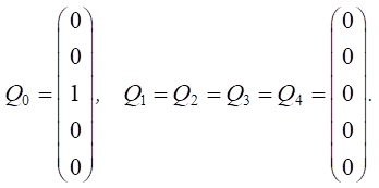
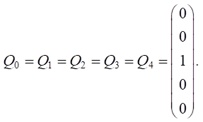
Let us set the vector of external pulses. Feed additives were introduced only in the first year, so we set a positive pulse +1 at the top of v5 for Q0. For the remaining years, we did not set external impulses:
Let us calculate Rn, n  pulses:
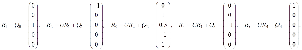
Figure 6 demonstrates how Rn pulses for the considered factors changed over time.
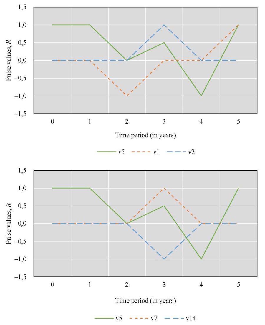
Fig. 6. Simulation results for Scenario 3
Scenario 4. Let us consider the specific efficiency of natural reproduction of commercial bream in the Tsimlyansk Reservoir when using feed additives annually for five years.
The cognitive map for this scenario is also described in Figure 6. Relationship matrix U is similar to Scenario 3.
Let us set the vector of external pulses (+1) at vertex v5 for each year of the simulation:
Let us calculate Rn, n  pulses:
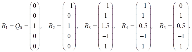
Figure 7 provides the results of the change in Rn pulses for the considered factors over time
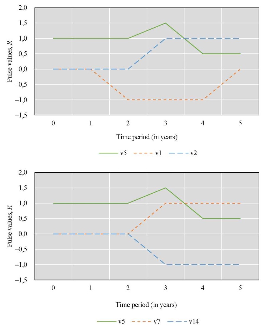
Fig. 7. Simulation results for Scenario 4
Discussion. In summary, the first two scenarios reflect the impact of removing an invasive species, zebra mussels, from the bottom of a reservoir. In the first scenario, the cleaning process was carried out only during the first year of the study. In the second scenario, it was conducted throughout the entire three-year simulation period. A comparison of the results suggests that annual removal of zebra mussels from the reservoir's bottom significantly improved water quality. Such anthropogenic impact made it possible to reduce the concentration of polluting biogenic substances (nitrogen, phosphorus, and silicon compounds). As a result, eutrophication in the reservoir decreased, overgrowth of aquatic vegetation, waterlogging, and natural aging decreased, and transparency of the water increased. However, positive effects of the one-time cleanup did not last for more than a year. Furthermore, from the second year to the third, the concentration of nitrogen, phosphorus, and silicon compounds would continue to increase if zebra mussels were not removed from the bottom of the reservoir.
Visualization of the simulation results for the second scenario (Fig. 4) showed that the annual cleaning of the bottom of the Tsimlyansk Reservoir over three years significantly improved the quality of waters of the Tsimlyansk Reservoir. The effect was better than in the first scenario, as the pulse of the waters of the Tsimlyansk Reservoir continued to grow more intensively in the third year. In the third year, the pulse in Scenario 2 (Fig. 4) was 0.75, and in Scenario 1 (Fig. 3) it was 0.25. Similar to the first scenario (Fig. 3), the concentration of nutrients (Fig. 4) decreased during the first year. In the second year, the indicator increased, but not as sharply and significantly as in the first scenario, that is, with a single bottom cleaning. For the second scenario, there was no symmetry between the graphs of anthropogenic impact and the concentration of biogenic substances. Thus, annual cleaning of the reservoir bottom from zebra mussels was more effective for improving the water condition and less effective for the concentration of nutrients.
The second set of scenarios focused on the ichthyological aspects of the artificial reservoir. They considered the impact of fish feeding on the spawning population, the annual replenishment of juveniles, the level of commercial exploitation of fish biological resources and the eutrophication of the reservoir were considered. In the first case, additional feeding was used only in the first year of modeling, while in the second scenario it was applied throughout the entire five-year period. One-time feeding had a positive impact on juvenile population growth and commercial exploitation, reducing eutrophication but not achieving sustainable results. Continuous feeding could significantly increase juvenile numbers and reduce eutrophication levels, leading to increased fishing.
According to the data presented in Figure 6, during the first year, additional feeding had no significant effect on the replenishment of juvenile fish, the level of commercial fishing, or the level of eutrophication in the reservoir. This suggests that there was a delayed effect. During the second year, however, there was an increase in the number of spawning fish and both the annual replenishment of juvenile fish and commercial fishing increased. Due to the active fishing during the third year, the volume of juvenile fish being replenished decreased. These factors were interrelated, leading to a decrease in commercial fishing at the same time. The eutrophication of the reservoir decreased during the second year. This can be explained by the fact that with an increased fish population, algae are consumed faster, which leads to smaller juvenile fish, a decline in the spawning population, and as a result, less algae consumption, and an increase in eutrophication during the third year. During the fourth year, there was no increase in the schedules for the replenishment of juvenile fish or eutrophication. The improvement in the condition of the spawning area can be attributed to the growth of juvenile fish.
From the graphs in Figure 7, we can conclude that the condition of the reservoir would change significantly if the additional feeding was extended for five years. During the first three years, the results were similar to those of Scenario 3. However, there was a notable improvement in the annual replenishment of juvenile fish and an increase in the commercial exploitation of fish biological resources. At the same time, there were no obvious cyclical patterns of increase and decrease in fish numbers, as observed in the modeling results of the sixth scenario. The decline in the spawning population before the fourth year may be attributed to increased commercial exploitation. By the fifth year, however, the situation improved, likely due to the growth of juvenile fish. The growing population of fish contributed more to the cleaning of the reservoir by eating more vegetation, leading to a noticeable reduction in eutrophication.
Figures 6 and 7 show the same pulse from feeding fish for the first year, calculated according to formula (1). In the second year, the pulse in Scenario 3 (Fig 6) dropped to 0. Scenario 4 (Fig. 7) reflected the resumption of feeding, so the pulse reached 1, and then increased due to the cumulative effect and the effect of feeding on related factors. The development of this situation led to the fact that there were more juveniles, they needed more food, and feeding no longer gave such a significant pulse.
To interpret the results, it was important to take into account that, according to formula (1), a decrease in pulse (if its value is positive) did not contradict an increase in the value of the corresponding factor. Thus, Figures 6 and 7 mathematically reflect the biological processes under study.
Based on the results obtained, it is possible to judge how to ensure the sustainable ecological development of the Tsimlyansk Reservoir. This requires annual environmental monitoring and measures to reduce anthropogenic impact (with a mandatory assessment of the economic component).
Conclusion. The proposed graph model includes 20 factors (concepts) that significantly affect the water quality and biological productivity of the Tsimlyansk Reservoir. The solution was created in the absence of sufficient expert information and with a rarely updated database of indicators. The matrix of weighting coefficients corresponding to the proposed graph model was based on expert estimates, which may be subjective and may change over time. Additionally, when aggregating data, there is a possibility of errors in estimating the pulse values. Within the framework of the chosen scenario approach, the proposed graph model allows for the incorporation of new information and quick, low-cost analysis of the effectiveness of proposed measures to improve the ecological state of the reservoir.
The results of the study can be used to assess the economic impact and damage caused by human activities on aquatic ecosystems. Ideally, these ecosystems should strive for a state of homeostasis.
To improve the presented model, it is necessary to fine-tune the weighting coefficients. This should take into account nonlinear and threshold effects as well as other relevant indicators.
1. The Tsimlyansk Reservoir and Reservoirs of the Lower Don Basin. Federal Agency for Water Resources. (In Russ.) URL: https://voda.gov.ru/activities/tsimlyanskoe-vodokhranilishche-i-vodokhranilishcha-basseyna-nizhnego-dona/?sphrase_id=177953&PAGEN_1=2 (accessed: 27.09.2025).
2. The Quality of Surface Waters of the Russian Federation. Yearbook-2023. Rostov: Roshydromet, Hydrochemical Institute; 2024. 156 p. ISBN (In Russ.)
3. Strategy of Socio-Economic Development of the Rostov Region for the Period up to 2030. Decree of the Government of the Rostov Region No. 864 dated December 26, 2018. As amended by No. 1100 dated December 19, 2022). The Ecology Section. The Official Portal of the Government of the Rostov Region. (In Russ.) URL: https://www.donland.ru/activity/2158/#pril435 (accessed: 28.10.2025).
1. Gerasimov YuV, Malin MI, Solomatin YuI, Kosolapov DB, Lazareva VI, Sabitova RZ, et al. Results of a Comprehensive Study of the Structure and Functioning of Ecosystems of the Volga Reservoir Cascade in 2017. In: Proceedings of the Conference “Expeditionary Research on Research Vessels of the Federal Agency for Scientific Organizations of Russia and the Spitsbergen Archipelago in 2017”. Sevastopol: Marine Hydrophysical Institute of the Russian Academy of Sciences; 2018. P. 178–187. (In Russ.)
2. Belova YuV, Nikitina AV. Application of Methods of Observational Data Assimilation to Model the Spread of Pollutants in a Reservoir and Manage Sustainable Development. Safety of Technogenic and Natural Systems. 2024;8(3):39–48. https://doi.org/10.23947/2541-9129-2024-8-3-39-48
3. Wantzen KM, Rothhaupt K-O, Mörtl M, Cantonati M, G.-Tóth L, Fischer P. Ecological Effects of Water-Level Fluctuations in Lakes. Hydrobiologia. 2008;613:1–4. https://doi.org/10.1007/s10750-008-9466-1
4. Minina LM, Minin AE, Moiseev AV. Influence of the Dynamics of Water Levels in Spring on the Area Spawning Grounds and Efficiency of Natural Reproduction Limnophilic Fish Species of the Cheboksary Reservoir. Trudy VNIRO. 2021;185:84–93. (In Russ.) https://doi.org/10.36038/2307-3497-2021-185-84-93
5. Logez M, Roy R, Tissot L, Argillier C. Effects of Water-Level Fluctuations on the Environmental Characteristics and Fish-Environment Relationships in the Littoral Zone of a Reservoir. Fundamental and Applied Limnology. 2016;189(1):37–49. https://doi.org/10.1127/fal/2016/0963
6. Belova YuV, Rahimbaeva EO, Litvinov VN, Chistyakov AE, Nikitina AV, Atayan AM. The Qualitative Regularities of the Eutrophication Process of a Shallow Water Research Based on a Biological Kinetics Mathematical Model. Bulletin of the South Ural State University. Ser. Mathematical Modelling, Programming & Computer Software. 2023;16(2):14–27. (In Russ.) https://doi.org/10.14529/mmp230202
7. Moiseenko TI. Aquatic Ecotoxicology: Theoretical Principles and Practical Application. Water Resources. 2008;35(5):530–541. https://doi.org/10.1134/S0097807808050047
8. Shibaev SV. Commercial Ichthyology. Saint Petersburg: Prospekt Nauki; 2024. 399 p. (In Russ.) URL: https://www.iprbookshop.ru/79996.html (accessed: 30.08.2025).
9. Strayer DL. Alien Species in Fresh Waters: Ecological Effects, Interactions with Other Stressors, and Prospects for the Future. Freshwater Biology. 2010;55:152–174. https://doi.org/10.1111/j.1365-2427.2009.02380.x
10. Alimov AF, Bogutskaya NG. Biological Invasions in Aquatic and Terrestrial Ecosystems. Monograph. Moscow: Limited Liability Company Scientific Publications Partnership KMK; 2004. 436 p. (In Russ.)
11. Zviagintsev AYu, Guk YuG. Estimation of Ecological Risk Arising from Bioinvasion in Marine Coastal Ecosystems of Primorye Region (with Sea Fouling and Ballast Waters as an Example). Izvestya TINRO. 2006;145:3–38. (In Russ.)
12. Lazareva VI, Sabitova RZ. Zooplankton of the Tsimlyansk Reservoir and Volga–Don Shipping Canal. Zoologicheskii Zhurnal. 2021;100(6):603–617. (In Russ.) https://doi.org/10.31857/S0044513421040115
13. Persson L, De Roos AM, Claessen D, Byström P, Lövgren J, Sjögren S, et al. Gigantic Cannibals Driving a Whole-Lake Trophic Cascade. Proceedings of the National Academy of Sciences. 2003;100(7):4035–4039. https://doi.org/10.1073/pnas.0636404100
14. Sukhinov AI, Chistyakov AE, Belova YV, Nikitina AV, Sumbaev VV, Semenyakina AA. Supercomputer Modeling of Hydrochemical Condition of Shallow Waters in Summer Taking into Account the Influence of the Environment. Communications in Computer and Information Science. 2018;910:336–351. https://doi.org/10.1007/978-3-319-99673-8_24
15. Williams RJ, Martinez ND. Simple Rules Yield Complex Food Webs. Nature. 2000;404:180–183. https://doi.org/10.1038/35004572
16. Urban D, Keitt T. Landscape Connectivity: A Graph-Theoretic Perspective. Ecology. 2001;82(5):1205–1218. https://doi.org/10.1890/0012-9658(2001)082[1205:LCAGTP]2.0.CO;2
17. Dambacher JM, Hang‐Kwang Luh, Hiram W Li, Rossignol PA. Qualitative Stability and Ambiguity in Model Ecosystems. The American Naturalist. 2003;161(6):876–888. https://doi.org/10.1086/367590
18. Perevaryukha AYu. Graph Model of Interaction of Anthropogenic and Biotic Factors for Productivity of the Caspian Sea. Vestnik of Samara University. Natural Science Series. 2015;21(10):181–198. (In Russ.) https://doi.org/10.18287/2541-7525-2015-21-10-181-198
19. Golokolenova TB. Dynamics of the Phytocenosis of the Upper Reach of the Tsimlyansk Reservoir. In: Proceedings of the XVII International Scientific-Practical Conference “Problems of Sustainable Development and Ecological and Economic Security of Regions”, Volzhsky, April 27–28, 2023. Volgograd: Sfera; 2023. P. 145–149. (In Russ.)
20. Kochetkova AI, Bryzgalina ES, Kalyuzhnaya IY, Sirotina SL, Samoteyeva VV, Rakshenko EP. Overgrowth Dynamics of the Tsimlyanskoe Reservoir. Principles of the Ecology. 2018;1:60–72. (In Russ.) https://doi.org/10.15393/j1.art.2018.7202
21. Chistyakov AE, Kuznetsova IYu. Assessment of Environmental Risks of a Shallow Water Body during Dredging Works. Safety of Technogenic and Natural Systems. 2024;2:37–46. https://doi.org/10.23947/2541-9129-2024-8-2-37-46
22. Dudkin SI, Leontiev SYu, Mirzoyan AV. The State of Stocks and Catches of Commercial Fish Species of the Azov and Black Seas for the Period 2000–2020: Dynamics and Trends. Trudy VNIRO. 2024;195:35–44. (In Russ.) https://doi.org/10.36038/2307-3497-2024-195-35-44
23. Heinle A, Slawig T. Internal Dynamics of NPZD Type Ecosystem Models. Ecological Modelling. 2013;254:33–42. https://doi.org/10.1016/j.ecolmodel.2013.01.012
24. Litvinov VN, Chistyakov AE, Nikitina AV, Atayan AM, Kuznetsova IY. Mathematical Modeling of Hydrodynamics Problems of the Azov Sea on a Multiprocessor Computer System. Computer Research and Modeling. 2024;16(3):647–672. (In Russ.) https://doi.org/10.20537/2076-7633-2024-16-3-647-672
25. Revutskaya OL, Frisman EY. Harvesting Impact on Population Dynamics with Age and Sex Structure: Optimal Harvesting and the Hydra Effect. Computer Research and Modeling. 2022;14(5):1107–1130. (In Russ.) https://doi.org/10.20537/2076-7633-2022-14-5-1107-1130
26. Abakumov AI, Izrailsky YuG. The Harvesting Effect on a Fish Population. Mаthematical Biology and Bioinformatics. 2016;11(2):191–204. (In Russ.) https://doi.org/10.17537/2016.11.191
Inna Yu. Kuznetsova, Senior Lecturer of the Department of Mathematics and Computer Science
ElibraryID: 650783
ScopusID: 57217115003
1, Gagarin Sq., Rostov-on-Don, 344003
Inna Yu. Kuznetsova, Senior Lecturer of the Department of Mathematics and Computer Science
ElibraryID: 772685
ScopusID: 57190226179
1, Gagarin Sq., Rostov-on-Don, 344003
The paper presents a graph model of the state of a large reservoir, which describes the interaction between anthropogenic and biotic factors of an ecosystem. The model demonstrates the dynamics of water quality under various modes of reservoir treatment, as well as evaluates the impact of fish feeding on population reproduction. The method allows for predicting the consequences of management decisions regarding reservoirs, and the results can be applied in planning fisheries and environmental management measures.
Kuznetsova I.Yu., Nikitina A.N. Study of Artificial Reservoir's Bioproductivity Based on a Graph Model of Natural and Anthropogenic Factor Interaction. Safety of Technogenic and Natural Systems. 2025;9(4):305-318. https://doi.org/10.23947/2541-9129-2025-9-4-305-318. EDN: OBWTCN


Safety of Technogenic and Natural Systems
eISSN 2541-9129
Contact with: Publisher / Editorial Office of the Journal
Publisher: Don State Technical University - DSTU, Rostov-on-Don, Russia - https://donstu.ru/en/
Editor-in-Chief: Meskhi Besarion Chokhoevich, Doctor of Technical Sciences, Professor (Rostov-on-Don, Russia)
Don State Technical University
1, Gagarin Sq., Rostov-on-Don, 344003, Russia
tel.: +7 (863) 2738-372, e-mail: btps@donstu.ru
1, Gagarin Square, Rostov-on-Don, 344003, Russian Federation, Don State Technical University
Processing of personal data


